The Burr Distribution. [1].
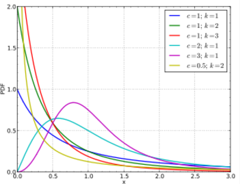
The Burr distribution (also called the Burr Type XII distribution or Singh–Maddala distribution) is a unimodal family of distributions with a wide variety of shapes. It is obtained by transforming a Pareto distribution, raising it to a positive power. Restricting the Burr distribution’s parameters in a certain way will result in the paralogistic distribution [1].
The distribution is used to model a wide variety of phenomena including crop prices, household income, option market price distributions, risk (insurance) and time to destination. It is particularly useful for modeling histograms.
Types I to XII
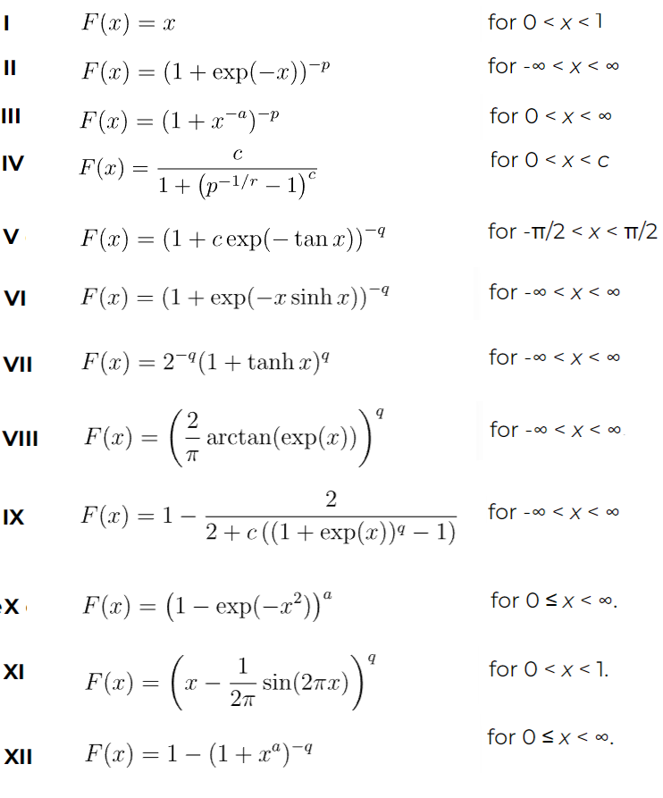
In 1941, Burr introduced twelve cumulative distribution functions (CDFs) that could be fit to real life data. However, the Burr Type XII family was the only one he originally studied in depth; the others were studied in depth at later dates. Thus, the term “Burr distribution” usually refers to type XII.
Burr Type III (also called the inverse Burr distribution or Dagum type distribution) is (along with type XII) commonly used for statistical modeling. To obtain this distribution from the PDF of the Burr type II: replace “X” in the PDF with “ln(x)” [2].
Burr Type IV: When the location parameter (l) = 0 and scale parameter (s) = 1, it becomes the standard Burr type VI distribution.
A five-parameter distribution, the beta Burr XII, is useful for modeling lifetime data. It is called the Singh–Maddala distribution in economics.
Most forms of this distribution have little research associated with them. For example, Feroze et. al [3] say about the Type V that “Many properties of the parameters of the distribution under different estimation procedures are still to be revealed.” Thus, the CDFs for these types can be challenging to track down. Credit to John D. Cook [4] for finding the CDFs for all 12:
The Burr distribution Type XII is the most common Type you’ll come across, thus I’ll dive in deeper here to its properties. It is defined by the following parameters:
c and k: shape parameters. For Burr Type XII, these are both positive. Type III has a negative c parameter.
When the fourth parameter, γ, equals zero, it gives a three parameter (c, k, α) distribution.
A given set of data can be matched to a Burr distribution by matching the mean, kurtosis, skewness and variance of the data set.
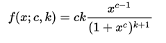
The probability density function (pdf)) for the Burr distribution (Type XII) is:
Compound Weibull distribution with a gamma distribution as its shape parameter [5]: The Burr distribution is simpler to use and understand than this compound Weibull (sometimes called the generalized Burr distribution), but it is less flexible due to one less parameter.
Gamma distribution: The Burr distribution is a more versatile distribution than the one-parameter gamma distribution. However, the gamma distribution is easier to understand and use.
The paralogistic distribution emerges from the Burr distribution when the shape parameter, k, is set to 2. The sigmoidal shapes distribution is often observed in biological and social phenomena.
J-shaped beta distribution: This is a special case of the beta distribution with a J-shaped density.
user:Arthena, CC BY-SA 4.0 <https://creativecommons.org/licenses/by-sa/4.0>, via Wikimedia Commons
Johnson, N.L. et. al (1995). “Continuous Univariate Distributions”. Vol. 2, John Wiley & Sons, New York, NY, USA, 2nd edition.
Feroze, N. & Aslam, M. (2013) “Maximum Likelihood Estimation of Burr Type V Distribution under Left Censored Samples.” WSEAS Transactions on Mathematics.
Cook, J. The Other Burr Distributions: https://www.johndcook.com/blog/2023/02/15/all-burr-distributions/
Muhammed, H. BIVARIATE GENERALIZED BURR AND RELATED DISTRIBUTIONS: PROPERTIES AND ESTIMATION. Journal of Data Science,17(3). P. 535 -550,2019. DOI:10.6339/JDS.201907_17(3).0005
Comments? Need to post a correction? Please Contact Us.
 The Burr distribution Type XII is the most common Type you’ll come across, thus I’ll dive in deeper here to its properties. It is defined by the following parameters: