< Probability Distributions > Beta Distribution
Contents:
What is a Beta Distribution?
The beta distribution (also called the beta distribution of the first kind) is a family of continuous probability distributions defined on [0, 1]. This distribution is similar to the binomial distribution, except where the binomial models the number of successes (x), the beta models the probability (p) of success.
A beta distribution is a versatile way to represent outcomes for percentages or proportions. For example, how likely is it that a rogue candidate will win the next Presidential election? You might think the probability is 0.2. Your friend might think it’s 0.15. The beta distribution gives you a way to describe this. One reason that the beta distribution can be confusing to work with is that there are three “Betas” to contend with, and they all have different meanings:
-
-
- Beta(α, β): the name of the probability distribution.
- B(α, β ): the name of a function in the denominator of the pdf. This acts as a “normalizing constant” to ensure that the area under the curve of the pdf equals 1.
- β: the name of the second shape parameter in the pdf.
-
The basic beta distribution is also called the beta distribution of the first kind. Beta distribution of the second kind is another name for the beta prime distribution.
Properties
The general formula for the probability density function (pdf) is: 
where:
-
-
- α and β are two positive shape parameters which control the shape of the distribution.
-
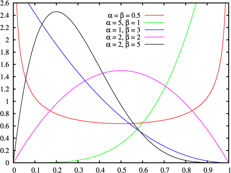
The graph of the beta density function can take on a variety of shapes. For example, if α < 1 and Β < 1, the graph will be a U shaped distribution, and if α = 1 and Β = 2, the graph is a straight line.
The general formula for the cumulative distribution function (CDF) is: 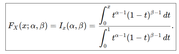 which includes the regularized beta function:
Software Options
Most software packages have options for the beta distribution.
Implement a beta distribution by typing BetaDistribution[alpha,beta].
R
dbeta(x, shape1, shape2, ncp = 0, log = FALSE) pbeta(q, shape1, shape2, ncp = 0, lower.tail = TRUE, log.p = FALSE) qbeta(p, shape1, shape2, ncp = 0, lower.tail = TRUE, log.p = FALSE) rbeta(n, shape1, shape2, ncp = 0)
where:
-
-
- x, q = vector of quantiles. p = vector of probabilities.
- n = # of observations.
- shape1, shape2 = shape parameters α and β
- ncp = non-centrality parameter.
- log, log.p = logical; if TRUE, probabilities p are given as log(p).
- lower.tail = logical; if TRUE (default), probabilities are P[X ≤ x], otherwise, P[X > x].
-
Excel Beta Distribution: BETA.DIST & INV.BETA
Watch the video for an example of BETA.DIST:

-
-
- The value where you want to evaluate the function.
- Alpha and Beta, the parameters of the distribution which determine shape.
- The lower and upper bound.
-
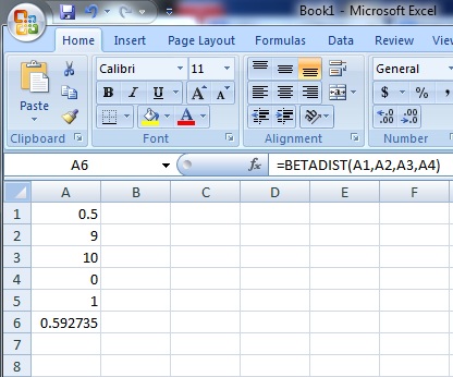
An extra input is needed for the Excel 2010 Beta Distribution: cumulative. Cumulative is a logical value that determines the function’s form and can either be TRUE (returns the cumulative distribution function) or FALSE (returns the probability density function). Example problem: Calculate a cumulative distribution function for a beta distribution in Excel at 0.5 with an alpha of 9, a beta of 10, a lower bound of 0 and an upper bound of 1.
Excel 2007 and Earlier:
-
-
- Type the value where you want to evaluate the function in cell A1. For this example, type “.5” in cell A1.
- Type the value for alpha in cell A2 and then type the value for beta in cell A1. For this example, type “9” in cell A2 and then type “10” in cell A3.
- Type the lower bound in cell A4 and then type the upper bound in cell A5. For this example, type “0” in cell A4 and then type “1” in cell A5
- Type the beta distribution function into cell A6. The format of the function is =BETADIST(value,alpha,beta,lower bound,upper bound). For this example, type “=BETADIST(A1,A2,A3,A4,A5)” into cell A6. Press “Enter” to see the result for the beta distribution, which is 0.592735.
-
Excel 2010 and later
Excel 2010 and later uses the BETA.DIST function. If you’re using earlier versions, use BETADIST instead. Inputs are as follows:
-
-
- A value where you want to evaluate the function.
- Alpha (α) and Beta (β), which determine the distribution’s shape.
- The lower and upper bound.
- “Cumulative” — a logical value (TRUE/FALSE) that determines the function’s form. TRUE returns the CDF and FALSE returns the PDF.
-
Example problem: Calculate a cumulative distribution function for a beta distribution at 0.5 with α = 9, β = 10, lower bound = 0 and upper bound = 1.
Applications of the Beta Density Function
The beta distribution is used for a variety of applications for modeling the behavior of random variables limited to intervals of finite length. Uses include:
-
-
- Bayesian inference, as the conjugate prior probability distribution for the Bernoulli, binomial, geometric and negative binomial distributions.
- The Rule of Succession (such as Pierre-Simon Laplace’s treatment of the sunrise problem),
- Task duration modeling.
- Project/planning control systems like PERT and CPM.
- In project management for the “three-point technique,” (also called the beta distribution technique), which recognizes uncertainty in estimated project time [1]. The three-point estimation technique is used to account for uncertainty in project time estimates. By applying this method, project managers can leverage powerful quantitative tools to identify tasks with the highest risk. It also facilitates effective management of overall project completion time.
-
References