Probability Distributions > Folded Normal Distribution
Contents:
What is a Folded Normal Distribution?
The folded normal distribution is defined as the absolute value of the normal distribution [1]. It can be used to describe what happens when only the magnitude of a random variable is recorded, but not its sign. The name comes from the fact that the negative half of the density of the normal distribution on (−∞,0] is folded over
to the positive half on [0,∞).
Folded normal distribution properties
The mean( μ) and variance (σ2) of X in the original normal distribution becomes the location parameter (μ) and scale parameter (σ) of Y in the folded distribution. A more formal definition uses these two facts:
If Y is a normally distributed random variable with mean μ (the location parameter) and variance σ2 (the scale parameter), that is, if Y ∼ N μ,σ2, then the random variable X = |Y | has a folded normal distribution.
The probability density function (PDF) is given as follows: Suppose that a random variable Y ~ N (μ, σ2) is a normally distributed with mean μ and variance σ2. Let X = |Y|. Then X has a folded normal distribution with PDF [2]
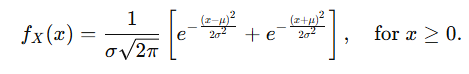
Where σ2 and μ are the scale parameter and location parameter for the parent normal distribution (they become the shape parameters for the folded normal distribution).
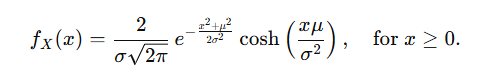
Alternatively, the PDF can be expressed as a function of the hyperbolic cosine function cosh by taking z as z = (y – μ)/σ:
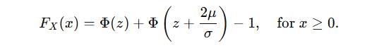
The cumulative distribution function (CDF) can be written as
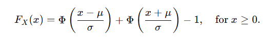
Taking z = (x – μ) / σ , the CDF can also be expressed as:
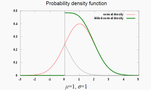
Graph of the folded normal
The graph below shows an example of how this continuous distribution looks. The probability mass to the left of x = 0 is folded over by taking the absolute value of x (represented in green).

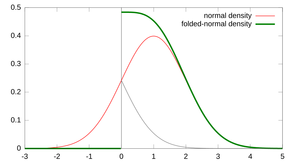
Note that although it’s called a folded normal distribution, it is not what you would get if you drew a normal distribution on a sheet of paper and folded it in half — although its close! That’s because we’re interested in taking the absolute values on the left half of the distribution (less than x = 0) and folding those values over to the right — so it’s more like folding in cooking — where two components (such as eggs and flour) are combined.
The mean (μ) and variance (σ2) of X in the original normal distribution become the location parameter (μ) and scale parameter (σ) of Y in the folded distribution. A more formal definition uses these two facts:
If Y is a normally distributed random variable with mean μ (the location parameter) and variance σ2 (the scale parameter), that is, if Y ∼ N μ,σ2, then the random variable X = |Y | has a folded normal distribution.
Ahsanullah et al. [2]
The shape of this graph reflects some interesting properties about how data behaves in relation to each other in real-world scenarios – for example, in many cases it may be more useful to know only whether a given value exceeds some threshold, rather than both its direction and extent relative to that threshold (e.g., when measuring changes in stock prices). By folding over at zero, we no longer need to consider negative values separately from positive values – instead they are combined into one single value which can be compared against other data points or thresholds more easily.
Furthermore, by folding over at zero we also shift our focus away from any particular point on the graph – instead we are looking at how much total area lies above or below any given point on the graph (i.e., what percentage of all possible outcomes lie above or below that point). This allows us to make statements about likelihoods based on these areas under curves – for example, “what is the probability that my random variable exceeds some threshold?”
Folded normal distribution calculator
This calculator allows you to create a CDF of the folded normal distribution and change the parameters of the function. You can also calculate the median and the first and third quartiles.
The Half-Normal Distribution
![Probability density function (PDF) of the half normal distribution with standard deviation 1/2 [1].](https://www.statisticshowto.com/wp-content/uploads/2015/08/half-normal-distribution-pdf-1.png)
The half normal distribution is the distribution of the absolute value of a normally distributed random variable. It is a special case of the folded normal and truncated normal distributions. The probability density function is 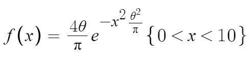
Where the mean is zero and the standard deviation is 1/θ [2]. The folded normal distribution is also defined as the distribution of the absolute value of a normally distributed random variable, which means that the folded normal distribution only considers the positive values of the normal distribution.
However, the half-normal distribution is a special case where the mean (μ) of the normal distribution is zero; in other words, when μ = 0, the folded normal distribution becomes the half-normal distribution. Thus, it could be more aptly called the “half standard normal” distribution.
Applications of the half normal distribution
The half normal distribution has some useful applications, such as modeling measurement and lifetime data. In fact, this is one of the most important variations of the folded normal, because you’re more likely to be interested in normal distributions with a mean of 0 (i.e. a standard normal). For example, the half-normal distribution models Brownian motion — the random movement of microscopic particles suspended in a liquid or gas.
Another application for which this type of distribution can be used is in modeling measurement data. Measurement data can often be skewed or contain outliers that make it difficult to model accurately. By using a half-normal distribution, however, one can easily identify these anomalies and create an accurate model for the data that excludes these outliers.
The half-normal distribution can also be used to model lifetime data, such as when analyzing failure rates in components or products over time. By using this type of distribution, one can determine how many failures are expected over a certain period of time and use this information to plan accordingly.
References
- Kumbhaker, S. et al. (2015). A Practitioner’s Guide to Stochastic Frontier Analysis Using Stata. Cambridge University Press.
- Ahsanullah, M. et al. (2014). Normal and Student ́s T Distributions and Their Applications. Atlantis Press.
- Half-normal distribution. Retrieved September 6, 2023 from: https://archive.lib.msu.edu/crcmath/math/math/h/h026.htm