Loglinear Model (Log Linear Distribution): Definition, Uses

Probability distributions > Loglinear model / distribution

A log linear distribution (or loglinear model) is a discrete probability distribution that is typically used to analyze relationships between two or more categorical variables. When it is used to model cell counts in contingency tables, it is sometimes called a Poisson regression.  A logarithmic transformation is performed on the input data before it is fit into a linear equation. This transformation makes for more accuracy when predicting non-linear relationships.

Unlike other modeling methods, a loglinear model don’t distinguish between response and explanatory variables;  all variables in the model are treated as response variables. The log linear model is a good choice for Poisson, Multinomial or Product-Multinomial sampling when there is no clear distinction between the response and explanatory variables, or when there are more than two response variables. Multiple linear regression is not appropriate for this type of data in part because the constant variance assumption will be violated.

As an example, let’s say you surveyed a group of students to find out whether they had ever used alcohol, marijuana, or vapes. You want to know how the cell counts in the following table depend on the levels of categorical variables.

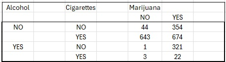
A loglinear model can help us understand the relationship between alcohol, marijuana, or vapes without having to define a specific response variable. On the other hand, if you wanted to create a model for two variables, such as vapes as a function of alcohol, you would could perform a logistic regression instead.

Parameterization of loglinear models

The loglinear model can take on many different parametrizations. Which form you use depends on your goal and what you’re using the distribution for. For example, let’s say you have a 3-way contingency table with variables X, Y, and Z. If you want to define a loglinear model for mutual independence, then you could define the formula as

log(m_ijk) = μ + λ^X_i + λ^Y_j + λ^Z_k = XYZ,

Where i, j, k are levels of categorical random variables X, Y, Z.

However, it’s unlikely you’ll be writing a formula for practical applications. Rather, you’ll be working with software functions such as the loglm() function in the MASS package of R.

Uses for the loglinear model

The loglinear model is widely used in a range of statistical and machine learning applications. For example:

• Contingency table analysis: Log linear models can be used to analyze contingency tables.  The models allow for tests of homogenous associations in I × J × K and higher-dimensional tables. Log linear models tell us how cell counts depend on the levels of categorical variables, modeling association and interaction patterms.
• Natural language processing: Log linear models can be used to analyze natural language data, such as text and code. For example, they can be used to find the frequency of specific words in a document or the frequency of distinct code segments within a program.
• Text mining: Log linear models can extract patterns and trends from text data. For example, they can identify commonly co-occurring words or frequently used constructs.

Poisson regression vs. log linear

Poisson regression is only used for numerical, continuous data. But the same technique can model categorical explanatory variables or counts in the contingency table cells. When used in this way, the models are called log linear models. Log-linear models determine the relationship between cell counts and the levels of categorical variables. They are designed to represent association and interaction patterns among categorical variables.

Log-linear modeling is well-suited for Poisson, Multinomial, and Product-Multinomial sampling. These models are particularly suitable when there isn’t a distinct separation between the response and explanatory variables or when multiple responses are present.

Other names for the loglinear model / distribution

Log-linear models haven many different names, depending on what field you’re working in [2]. For example:

1. Multinomial Logistic Regression is also called polytomous, polychotomous, multi-class logistic regression, or simply multilogit regression.
2. Maximum Entropy Classifier: Since logistic regression estimation adheres to the maximum entropy principle, it is occasionally termed “maximum entropy modeling,” with the resulting classifier called the “maximum entropy classifier.” This term was more common in natural language processing (NLP) literature in the 1990s; a more popular term today is the following neural network classification.
3. Neural Network – Single Neuron Classification: Binary logistic regression is equivalent to a single-layer, single-output neural network with a logistic activation function trained under log loss. This is sometimes called classification using a single neuron.
4. Generalized Linear Model and SoftNax Regression: Logistic regression is a generalized linear model featuring the logit link function. The logistic link function is occasionally referred to as SoftMax and, due to its use of exponentiation for converting linear predictors into probabilities, it is sometimes called an exponential model.

References

[1] Gross, B. & Berlin, M. Structure Learning.

[2] O’Connor, B. (2014). Lecture 8 Multiclass/Log-linear models, Evaluation, and Human Labels.