< List of probability distributions < Davis distribution
The Davis distribution is a family of continuous probability distributions named after American mathematician and statistician Harold T. Davis, who proposed the distribution to model income sizes in his 1941 monograph The Theory of Econometrics and Analysis of Economic Time Series [1]. It is a generalization of Planck’s radiation law from statistical physics. Both distributions can model the distribution of energy in a system, but the Davis distribution is more general and thus can model a wider range of systems.
The Davis distribution is — along with the Amoroso distribution — a member of D’Addario’s generating system of income distributions [2]. D’Addario’s system [3] is a translation system with flexible generating and transformation functions that encompass as many income distributions as possible:
- A generating function takes a random variable as input and returns a function of that random variable. It can be used to derive properties of the distribution such as the mean and variance.
- A transformation function takes a random variable and returns a new random variable. It can be used to change the shape of the distribution of the random variable.
Davis distribution PDF
The probability density function (PDF) of the Davis distribution is
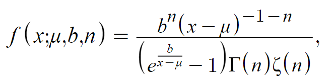
where
- Γ (n) = the Gamma function
- ζ(n) = the Riemann zeta function
- μ = a non-negative location parameter, which determines the location of the PDF on the x-axis.
- b = a positive, real-valued scale parameter,
- n = a positive, real-valued shape parameter > 1.
This unimodal distribution is defined over the interval (μ,∞). It is a fat-tailed distribution, which means that it decreases algebraically rather than exponentially for large x-values.
History of the Davis distribution
Davis cofounded the journal Econometrica and served as its Associate Editor for over two decades. He also worked on the staff of the non-profit Cowles Commission, which was founded in 1932 to support and encourage econometrics research.
Davis proposed his distribution to represent more than the upper tail of the distribution of income; he required a model with the following properties [2]:
- Subsistence income. f (x0) = 0, for some x0, which Davis described as the “wolf point,” as in it is the point at which the proverbial wolf enters the door.
- Existence of a modal income.
- For large values of x, the distribution approaches a Pareto distribution f(x)~A(x – x0)-α-1.
References
[1] Davis, H. T. (1941). The Analysis of Economic Time Series. The Principia Press, Bloomington, Indiana
[2] Kleiber & Kotz. (2003). Statistical Size Distributions in Economics and Actuarial Sciences. Wiley.
[3] D’Addario, R. (1949). Richerche sulla curva dei redditi. Giornale degli Economisti e Annali di Economia, 8, 91–114.