Probability Distribution List > Muth distribution
The Muth distribution, a model for non-negative continuous random variables, was introduced by Muth in 1977 [1].
The distribution has largely been overlooked in the statistical literature [2]; the distribution isn’t usually encountered in introductory probability and statistics courses. However, you’ll come across it in reliability theory, which deals with a system’s ability to function under certain conditions (like the effect of average time to repair) for a specified time period.
Pdf and characteristics of the Muth distribution
The shorthand X ∼ Muth(β) indicates that a random variable X has the Muth distribution with parameter β.
The probability density function (pdf) for the standard Muth distribution is:
f(x; β) = e βx – β) e -(1 / β)(e βx – 1) + βx
Where β is a shape parameter.
The distribution, which is based on a limited time interval, is flexible enough to fit a wide variety of lifetime datasets. It has several other notable characteristics:
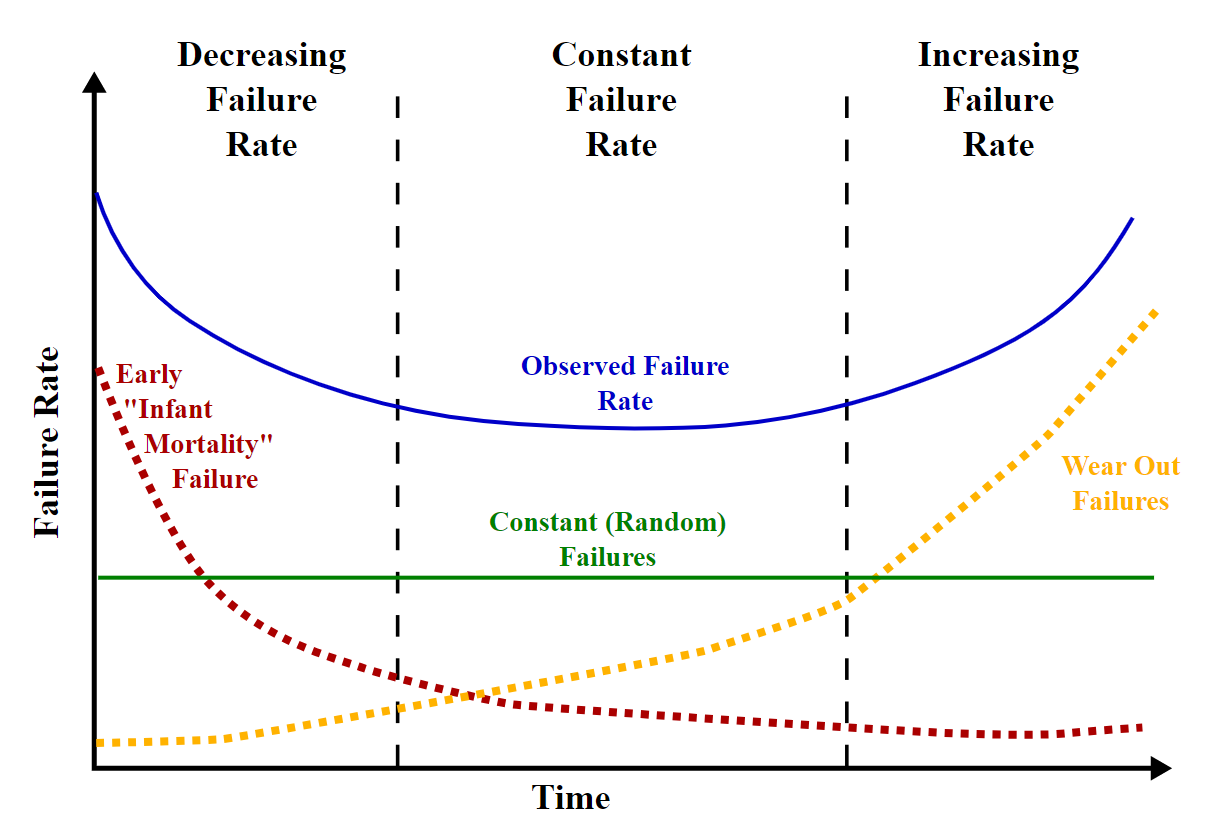
- It has the bathtub hazard function with a vertical asymptote [3].
- The distribution corresponds to the exponential distribution as β approaches zero.
- It’s tail is less weighted than other lifetime distributions such as the exponential, lognormal or Weibull.
- The inverse distribution function, median, moment generating function and characteristic function of X are not tractable (easily solvable).
History of the Muth distribution
The Muth distribution was first introduced by French biologist Teissier in 1934 [4]. Teissier considered the mortality of several domestic animal species resulting from pure ageing. Through empirical analysis, Teissier identified that animal mortality does not follow the human mortality pattern, as supported by the Gompertz law, frequently used in actuarial practice [5].
Laurent [6] later introduced a location version of Teissier’s distribution, characterizing it with life expectancy and exploring applications to demographic studies. Muth [7] observed that the Muth distribution displays a heavier tail, compared to well-known lifetime distributions such as the gamma distribution, lognormal distribution, and Weibull distribution. Rinne [8] used this model to estimate the lifetime distribution, expressed in kilometers, for a German data set based on used car prices. However, following Rinne’s work, Teissier’s distribution and its location version were forgotten and not referenced in available literature.
Leemis and McQueston [9] acknowledged and named the Muth distribution in their study of schematic representation in various univariate distributional relationships. In 2015, Pedro et al. reintroduced this distribution and its scaled version [10], studying its important properties through the exponential integral function.
References
Bathtub_curve.jpg: Wyattsderivative work: McSush, Public domain, via Wikimedia Commons
- J.E. Muth. (1977). Reliability models with positive memory derived from the mean residual life function. In C.P. Tsokos and I. Shimi (Eds.), The Theory and Applications of Reliability, volume 2, pp. 401–435. Academic Press, Inc., New York.
- Jodrá, P. & Arshad, M. (2021). An intermediate muth distribution with increasing failure rate. Communications in Statistics – Theory and Methods. Retrieved November 12, 2021 from: https://www.tandfonline.com/doi/abs/10.1080/03610926.2021.1892133?journalCode=lsta20
- Kosznik-Biernacka, S. (2007). Makeham’s Generalised Distribution. Computational Methods in Science and Technology 13(2), 113-120 from: http://citeseerx.ist.psu.edu/viewdoc/download?doi=10.1.1.552.4465&rep=rep1&type=pdf
- G. TEISSIER (1934). Recherches sur le vieillissement et sur les lois de la mortalité. II. essai d’interprétation genérale des courbes de survie. Annales de Physiologie et de Physicochimie Biologique, 10, pp. 260–284.
- B. GOMPERTZ (1825). On the nature of the function expressive of the law of human mortality, and on a new mode of determining the value of life contingencies. Philosophical Transactions of the Royal Society of London, 115, pp. 513–583.
- A. G. LAURENT (1975). Failure and mortality from wear and ageing – The Teissier model. In G. PATIL, S. KOTZ, J. ORD (eds.), A Modern Course on Statistical Distributions in Scientific Work, Springer, Heidelberg, vol. 17, pp. 301–320.
- J.E. Muth. (1977). Reliability models with positive memory derived from the mean residual life function. In C.P. Tsokos and I. Shimi (Eds.), The Theory and Applications of Reliability, volume 2, pp. 401–435. Academic Press, Inc., New York.