Lognormal Distribution: Definition, Examples

> Probability Distributions > lognormal distribution

What is a lognormal distribution?

A lognormal distribution is one where the logarithm of the variable of interest is normally distributed. Consequently, the lognormal variable itself is strictly positive (i.e., ) and often right-skewed.

This distribution is useful for modeling many real-world phenomena (e.g., infection incubation periods, mineral deposit sizes, financial returns under certain assumptions) that have positive support and significant skewness.

The reason that this distribution is called “log-normal” is that if X is a lognormally distributed random variable, then ln(X) follows a normal distribution. In simple terms: Imagine you have a random number $X$ that can only take positive values. When you look at the regular values of $X$ , it might form a long, stretched-out curve. However, if you switch to looking at the “log” of (which is like measuring how many times you multiply a small number to get $X$ ), that new set of numbers forms the familiar bell-shaped curve you see with a normal distribution. Because the log of is normal, we call itself log-normal.

Lognormal distribution properties

PDF

The probability density function (pdf) is defined by the mean μ and standard deviation, σ.

For a 2-parameter distribution, the pdf is

lognormal pdf

For three parameters, the pdf is

lognormal distribution 3 parameter pdf

Where:

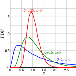
σ = the shape parameter. Also the standard deviation for the lognormal, this affects the general shape of the distribution. Usually, these parameters are known from historical data. Sometimes, you might be able to estimate it with current data. The shape parameter doesn’t change the location or height of the graph; it just affects the overall shape.
m = the scale parameter (this is also the median). This parameter shrinks or stretches the graph.
(or μ) = the location parameter, which tells you where on the x-axis the graph is located.

The standard lognormal distribution has a location parameter of 0 and a scale parameter of 1 (shown in blue in the image below). If Θ = 0, the distribution is called a 2-parameter lognormal distribution.

lognormal distribution function — A few examples of lognormal density functions [2].

2. Support:

2-parameters:
3 parameters:

3. Mean, Variance, Median, Mode

A big source of confusion with lognormal parameters arises because μ and σ are actually the mean and standard deviation of the underlying normal distribution ln⁡(X), not of X itself. Instead, the formulas are:

Mean = exp(μ + (σ² / 2)
Variance = exp(2μ + σ²) [exp(σ²) – 1]
Median (2-param) = exp (μ).
Mode (2-param) = exp(μ – σ²), if σ² < ∞.

For 3-parameters, replace x by x − θ in the formulas for the pdf and CDF, which depend on the variable x.

4. Skewness and Kurtosis

Skewness = (e^σ² + 2)√(e^σ² – 1)
Excess Kurtosis = e^4σ² + 2 e^3σ² + 3e^2σ² – 6.

5. MGF

M_X = E[e^tX]

The moment generating function (MGF) exists only for t in a limited range: for t < 1/σ² if μ ≠ 0.

5. CDF

The cumulative distribution function (CDF) is:

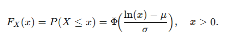
For the 3-parameter case, replace ln (x) with ln(x − θ).

When are lognormal distributions used?

A lognormal distribution often appears when a quantity is formed by multiplying many random factors (i.e., repeated random “shocks” that compound over time), leading to strictly positive values that can become very large. This process creates a distribution that is skewed to the right, meaning most observations cluster near smaller values but there is a long tail extending toward larger values. Consequently, many real-world data sets—such as certain biological measurements, some financial returns, and reaction times—have positive, skewed behavior consistent with a lognormal distribution.

For example, the following phenomenon can all be modeled with a lognormal distribution:

Milk production by cows.
Lives of industrial units with failure modes that are characterized by fatigue-stress.
Amounts of rainfall.
Size distributions of rainfall droplets.
The volume of gas in a petroleum reserve.

Many more phenomenon can be modeled with the lognormal distribution, such as the length of latent periods of infectious disease or species abundance [1].

Other Names for the Lognormal

Historically, the lognormal distribution has been called many names, including:

The Galton or Galton’s distribution (after the Victorian statistician Francis Galton).
Galton-McAlister distribution (McAlister was another Victorian statistician who published a description of the distribution with Galton).
Gibrat distribution, after the 20th century French economist who showed that the logarithms of certain economic variables (like factory distribution by number of workers) followed a normal distribution.
Cobb-Douglas distribution (after 20th century economists Charles Cobb and Paul Douglas). This term is used exclusively in economics, where it’s applied to production data.

Check out our YouTube channel for hundreds of probability and statistics help videos!

References:

Limpert, E. at al. (2001). Log-normal Distributions across the Sciences: Keys and Clues. BioScience. May / Vol. 51 No. Online: https://stat.ethz.ch/~stahel/lognormal/bioscience.pdf
Image: By Krishnavedala|Wikimedia Commons. CC 3.0.