Probability Distributions > Extreme Value Distribution & the Extreme Value Theory
Contents:
- What is an Extreme Value Distribution?
- Extreme Value Distribution Types I, II, and III
- The Generalized Extreme Value Distribution
- What is the Largest Extreme Value Distribution?
- What is an “Extreme Value?”
- Extreme Value Theory
What is an Extreme Value Distribution?
An extreme value distribution is a limiting model for the maximums and minimums of a data set. It models how large (or small) your data will probably get. For example, let’s say you wanted to build a levee to protect against storm surges. You can use historical storm data to create a limiting distribution that tells you how large the waves are likely to get and when the levee is probably going to fail. It may be helpful to think of the limit as a failure point — a point that, if exceeded, some kind of failure or end-of-life event will happen.
The basic idea is that three types of extreme value distributions (EVD Types I,II, and II) can model the extremes from any set of data, as long as the distribution is “well-behaved” (Gumbel, 1958), with the following characteristics:
- Is a continuous probability distribution. A continuous distribution has a range of values that are infinite, and therefore uncountable. For example, time is infinite: you could count from 0 seconds to a billion seconds…a trillion seconds…and so on, forever.
- Has an inverse. An inverse distribution is the distribution of the reciprocal of a random variable.
- Is made up of independent, identically distributed (IID) random variables. Identically Distributed means that there are no overall trends–the distribution doesn’t fluctuate and all items in the sample are taken from the same probability distribution. It’s basically the same thing as a random sample.
Extreme Value Distribution Types I, II, and III

If you generate any number of datasets, take the minimums and maximums from those sets, and generate a new distribution, it will follow one of three model types: no upper or lower limits (EVD I), bounded on the lower end (EVD II), or bounded on the upper end (EVD Type III) (Haan, 1977).
- EVD Type I: Gumbel Distribution (also called the Gumbel-Type). This is the most common EVD and has two forms: one for the minimum, and one for the maximum, although it is unbounded (not restricted to a range) and is defined on the entire range of real numbers. The probability density function has only one, unchanging shape which shifts according to the location parameter, μ. As μ increases, the distribution shifts to the left; As μ decreases, it shifts to the right. Let’s say you had a list of minimum pollution levels for the last decade. You could use the EVD Type I to model minimum pollution levels for the coming year. (More info: What is the Gumbel Distribution?)
- EVD Type II: Fréchet Distribution. This distribution is used to model maximum values in a data set . The Fréchet slowly converges to 1 and has three parameters: shape parameter, α, scale parameter, β and location parameter μ. It is defined on the interval μ ∞; In other words, it is bounded (restricted) on the lower side. A wide range of phenomena like flood analysis, horse racing, human lifespans, maximum rainfalls and river discharges in hydrology can be modeled with the Fréchet. (More info: What is the Fréchet Distribution?)
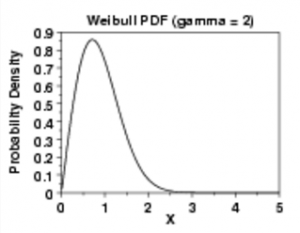
- EVD Type III: Weibull Distribution . The Weibull distribution is used in assessing product reliability to model failure times and life data analysis. The Weibull is actually a family of distributions that can take on many shapes, depending on what parameters you pick. It includes two exponential distributions, a right-skewed distribution and a symmetric distribution. (More info: What is the Weibull Distribution?)
The Generalized Extreme Value Distribution
The Generalized Extreme Value (GEV) distribution is a three-parameter distribution that unites the Type I (Gumbel), Type II (Fréchet) and Type III (Weibull) extreme value distributions. Which of the three models you choose depends upon the behavior in the tail of the parent distribution. However, you usually don’t know the behavior of the parent population’s tail (Holmes, 2015). If you don’t know anything about the tail behavior, then it’s impossible to choose which model might be the “best”. The GEV solves this problem by combining all three distributions into a single general form.
The CDF for the GEV is:

The parameters are:
- Location parameter, μ,
- Scale parameter, σ,
- Shape parameter, ξ.
σ and 1 + ξ(x-μ)/σ must be greater than zero. ξ and μ can take on any real value.
The shape parameter defines which distribution the generalized extreme value distribution takes on:
- When the shape parameter ξ is equal to 0, the GEV is equal to EVD Type I.
- When it is greater than 0, the GEV is equal to EVD Type II.
- When ξ is less than 0, the GEV is equal to EVD Type III.
The GEV distribution is sometimes called the Fisher–Tippett distribution, after Ronald Fisher and L. H. C. Tippett. However, this can cause a little confusion because the special case of the Gumbel distribution is also sometimes called the Fisher-Tippet distribution. To avoid the confusion, it’s best to refer to the distribution that encompasses all three types (EVD I,II & III) as the Generalized extreme value distribution.
What is the Largest Extreme Value Distribution?
The largest extreme value distribution another name for the Gumbel distribution.
The largest extreme value distribution is closely related to the smallest extreme value distribution: If a random variable X has a largest extreme value distribution, then the random variable −X has a smallest extreme value distribution, and the other way around.
What is an “Extreme Value?”

The term “extreme value” can mean something slightly different depending on where you read about it. Some authors use the term “extreme value” as another name for the minimum value and/or the maximum value of a function (i.e. the single smallest and/or largest number in the set), and others use as a synonym for an outlier. In calculus, the points where you find maximum and minimum values are called extrema, so some authors will refer to these points as “extreme values” as well. However, in most cases, when people talk about extreme values, they’re usually talking about values associated with the Extreme Value Theory.
What is the Extreme Value Theory?
Extreme Value Theory (EVT) is a branch of statistics dealing with stochastic behavior of extreme events found in the tails of probability distributions. A stochastic model represents a situation where uncertainty is present. In other words, it’s a model for a process that has some kind of randomness. EVT aims to predict probabilities for rare events greater (or smaller) than previous recorded events. For example, EVT might be used in seismology to predict the next mega-earthquake in California, the last of which was in 1857.
EVT originated from astronomy and the need to keep or reject outliers in data (Kotz & Nadarajah, 2003). Outliers are stragglers — extremely high or extremely low values — in a data set that can throw off your stats. For example, if you were measuring children’s nose length, your average value might be thrown off if Pinocchio was in the class. EVT has developed into a theory that is applicable to almost every area of science and business. For example, the theory can model and predict a diverse range of phenomena such as the maximum heights of ocean waves or the strength of financial markets (Coles, 2013). The theory, which uses extreme value distributions, is widely used in economics, finance, materials science, reliability engineering and many other fields.
Comparison to CLT
Extreme value theory is very similar to the Central Limit Theorem (CLT). Both theories involve limiting behaviors of distributions of independent and identically distributed random variables as n→ ∞, but there is a distinct difference: the CLT concerns the behavior of entire distributions of random variables, while extreme value theory only concerns the behavior of the tails of those distributions.
To put the difference between the EVT and CLT a little more precisely, the CLT describes the limiting behavior of X1, X2,…Xn while the extreme value theory describes the limiting behavior of the extremes max(X2,…,Xn) or min(X2,…,Xn) (de Haan & Ferreira, 2007).
Related Articles:
- The German Tank Problem finds population maximums, given sample maximums.
References
Caltech / Southern California Earthquake Data Center (2013). Fort Tejon Earthquake
Retrieved October 16, 2017 from: http://scedc.caltech.edu/significant/forttejon1857.html.
Coles, S. (2013). An Introduction to Statistical Modeling of Extreme Values. Springer Science & Business Media.
De Haan, L. & Ferreira, A. (2013). Extreme Value Theory: An Introduction. Springer Science and Business.
Fisher, R.A., Tippett, L.H.C. (1928). “Limiting forms of the frequency distribution of the largest and smallest member of a sample.” Proc. Cambridge Philosophical Society 24:180-190.
Gumbel, E. (1958). Statistics of Extremes. New York, Columbia University Press.
Haan, (1977). Statistical Methods in Hydrology. USGS.
Holmes, J. (2015). Wind Loading of Structures, Third Edition. CRC Press.
Kotz & Nadarajah, (2000). Extreme Value Distribution: Theory and Applications. World Scientific.
Weibull, W. (1951). “A statistical distribution function of wide applicability” J. Appl. Mech.-Trans. ASME 18(3), 293-297.