Complex analysis is the field of math which centers around complex numbers and explores the functions and concepts associated with them.
Negative square roots were first rejected as impossible and the name ‘imaginary’ was meant to exclude them from the serious mathematical study. However, complex numbers have turned up to be extremely useful in many branches of math and science. They play an important role in many areas of mathematics with practical applications in applied math, hydrodynamics, thermodynamics, and quantum mechanics. This makes it part of the bedrock underlying nuclear, electrical, aerospace and mechanical engineering.
The Basics
Contents (click to skip to that section):
Definitions & Functions in Complex Analysis
- Abelian Functions
- Abel’s Test: Definition & Example
- Branch Point
- Cartesian Form of complex numbers.
- Complex Conjugate: Definition, Properties
- Complex Modulus
- Contour Integral
- Entire Function (Integral)
- Essential Singularity
- Euler’s Totient Function / Phi Function: Simple Definition
- Exponential Integral Function
- Exterior Calculus
- Gauss Hypergeometric Function: Simple Definition
- H Function (Fox’s H-Function)
- Hankel Function
- Holomorphic Function (Analytic Function) & Universal Function
- Isotropic
- Laurent Series
- Meromorphic Function, Elliptic
- Möbius Function
- Non Trivial Zeros
- Pole (Isolated Singularity)
- Polylogarithm Function, Dilogarithm
- Punctured Disk
- Removable Singularity
- Sigma Function
- Univalent Functions
- Weierstrass Function
Complex Number Basics
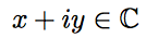
Complex numbers are numbers that are part real number and part imaginary number. The imaginary part is some multiple of the imaginary number, i (the square root of -1). Since the real and complex parts of these numbers are completely separable, they can also be considered to be ordered pairs of real numbers, representing points or vectors in R2.
We often write complex numbers as
Imaginary Numbers
- What is an Imaginary Number?
- The More Technical Definition.
- A Geometrical Interpretation of Imaginary Numbers.
- What are Imaginary Numbers Used For in Real Life?
- The History of Imaginary Numbers.
What is an Imaginary Number?
![]()
The idea of an imaginary number is relatively simple. All you really need to know for most math classes is that
i = √ -1.
The broader definition is:
An imaginary number is any number, that when squared, results in a negative number.
Sounds easy, right? The problem comes when you try and figure out which numbers are imaginary. Let’s take a few random numbers and square them to try and find one that’s imaginary (i.e. negative):
- 10 = 102 = 100
- .99 = .992 = 39801
- -4 = -42
- pi2 = .986960440109.
OK, none of those seem to be working. In fact, it’s almost impossible to “guess” an imaginary number. It would be like me asking you to guess what the word for “bicycle” is in Swahili. Or what the fifty-seventh digit in pi is. You’ll need to learn what they are, much in the same way that you learned what a “variable” is. Let’s take “x” for example. You probably know that “x” stands for “a variable.” Well, “i” stands for a very particular type of variable…an imaginary number. Unlike the variable x, which could be anything on the planet, i is equal to the square root of -1:
i = √-1
Now before you say “hang on…where did that come from? How do we know that i – √-1?”
Stop!
If you’re just learning about imaginary numbers, at this point it’s really important to take a deep breath, and accept that i = √-1. Remember learning about pi? The hardest thing was remembering it was equal to about 3.14. Then you got to use it to find circumferences and diameters of circles. And then, sometime down the road, you might have learned the history of pi and how it was derived. The imaginary number i is just like that. To reiterate what I said at the top of this section: all you need to know for most elementary math/algebra/statistics classes (and even a basic calc class) is that i = √-1.*
Back to Top
The More Technical Definition
You might see imaginary numbers defined this way: i2 = -1 (which is just i = √ -1 rewritten). You’ll be using the definition to try and solve equations. And if you’ve worked enough algebra equations you’ll know the first thing you do to an exponent is to get rid of it. How to get rid of it? By taking the square root of both sides. If you want to use the definition of i2, instead of √ 1, go ahead. For me, it makes equations more complicated. But if it works for you, there’s no reason at all why you can’t use it.
That said, there are some occasions when you’ll want to know some variations on i2 so that you can plug them into equations. Some you are likely to come across (and most of these are based on rules you probably already know, such as any number raised to zero is just one):
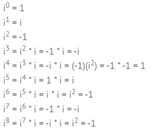
Take a look at that fourth term for a moment and notice it’s the same as i0. Do you see a pattern starting? The pattern continues (1, i, -1, i,) so that very high powers of i become relatively easy to work out. Odd powers like i20 will be equal to -1 or 1. Even powers like i57 are going to be equal to i or -i.
“i” raised to a negative exponent are seen less often, but they do exist (have a chuckle at that paradox!).
- i-1 = -i
- i-2 = -1
- i-3 = -i
A final note on the technical stuff: for basic algebra, the definition that i = √-1 works. But in more advanced classes (a complex numbers class, for example), you should know that –i is also a valid solution.
Back to Top
A Geometrical Interpretation of Imaginary Numbers
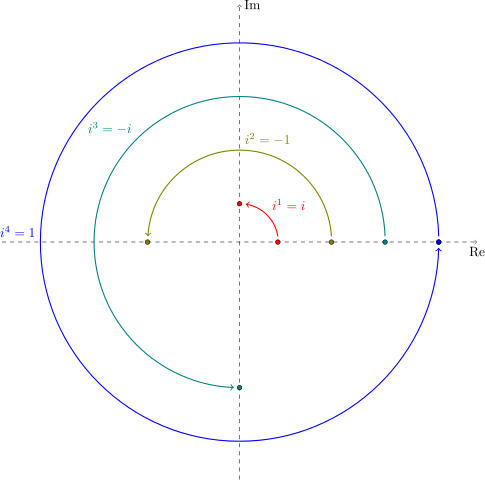
A complex number (a + bi) is just the rotation of a regular number. With a negative number, you count backwards from the origin (zero) on the number line. With an imaginary number, you rotate around the origin, like in the image above. The + and – signs in a negative number tell you which direction to go: left or right on the number line. In the same way, i tells you where to go on a Cartesian plane (well, it looks like a Cartesian plane, just that the y-axis is labeled i instead). Take the basic equation for i:
X2 = – 1
You can rewrite this as:
x * x = -1
Which is the same as saying:
What number, times itself is -1?
If you’re trying to think of a real number, like 2 or 3, remember that we’re working in a different real. If you have x * x = 4, you could use the number line to deduce that 2 * 2 = 4 by going right on the line 2 spaces and then 2 spaces. With imaginary numbers, you want to rotate, not multiply. If you rotate a number “x” 90 degrees and then 90 degrees again (which is x* x in the imaginary realm), you get -x.
If you find that hard to wrap your head around, let it sink in for a while. Consider this: not so long ago, people couldn’t comprehend negative numbers. In 1798, British mathematician said they “… darken the very whole doctrines of the equations and make dark of the things which are in their nature excessively obvious and simple.” Nowadays, every grade school student knows that a negative number is the opposite of a positive number.
What are Imaginary Numbers Used For in Real Life?
Right now, in the everyday world, imaginary numbers aren’t used. But imagine some day down the road, they might become part of our everyday language, much like the number zero has become commonplace (not so long ago, the number zero didn’t exist, but that’s a story for another article). If you become a mathematician, engineer or physicist, imaginary numbers become very important.
Imaginary numbers are mainly used in mathematical modeling. They can affect values in models where the state of a model at a particular moment in time is affected by the state of a model at an earlier time. You’re most likely to use imaginary numbers in fields like quantum mechanics and engineering where differential equations are used (differential equations are part of calculus). For example, they can be used to monitor the phase and amplitude of an audio signal or electrical currents. You’ll also come across these numbers in computer science, where some programming languages (like C#) use imaginary numbers in their routines. You’ll also come across them in advanced topics like Fourier Analysis.
The History of Imaginary Numbers
Heron of Alexandria (CE 100) is thought to be the first person proposing that the square root of a number (√63) could be a solution to a problem.
Niccolò Fontana (Tartaglia), Gerolamo Cardano and Lodovico Ferrari developed a formula in the early 16th century for finding the roots of cubic equations. Their work was published in the 1545 book Ars Magna. The formula included the roots of -1, which they realized didn’t exist. At the time, the numbers were called these non-existent numbers “numeri ficti.” Although they appeared in the equations, they ended up canceling out, so there was no need to figure out what they actually were. In 1572, Rafael Bombelli explained what the numeri ficti were and what they could be used for.
Rene Descartes came up with the phrase “imaginary numbers,” in the 17th century; mentioned in La Geometrie, it was meant to be a derogatory term. In the 18th century, the Swiss mathematician Leonhard Euler came up with the notation i as being equal to the square root of -1. Carl Friedrich Gauss popularized the use of imaginary numbers in the 19th century.
Complex Numbers vs. Imaginary Numbers
Complex numbers = Imaginary Numbers + Real Numbers
For example, 8 + 4i, -6 + πi and √3 + i/9 are all complex numbers.
Imaginary numbers and complex numbers are often confused, but they aren’t the same thing. Take the following definition:
“The term “imaginary number” now means simply a complex number with a real part equal to 0, that is, a number of the form bi.”
Some people read the first part of the sentence (bolded) to read that the two are equivalent. They aren’t: read the second part of the sentence carefully. What it is saying is:
- Take a random complex number like 7 + 4i.
- Make the “real” part of the equation zero. 0 + 4i.
That equals 4i, which is imaginary. In other words, you can get an imaginary number from a complex number. But they are not the same thing.
Back to Top
Complex Plane
A complex plane (also called an Argand diagram after the 18th century amateur mathematician Argand) is a two-dimensional graph of complex numbers. It gives mathematicians a graphical way to represent complex numbers instead of as an algebraic expression.
The graph of the complex plane looks almost identical to the usual xy-axis,
The x-axis on a complex plane represents the real part of a complex number and the y-axis represents the imaginary part. Therefore, they are most often labeled as “real axis” and “imaginary axis” instead of “x” and “y”, but you might also see other labels and notation used. But, no matter what variation appears on a graph, the giveaway that you’re looking at the complex plane (as opposed to a Cartesian plane) is the inclusion of “i”, either as an equation or as labeled steps on the y-axis.
How do you plot numbers on the complex plane?
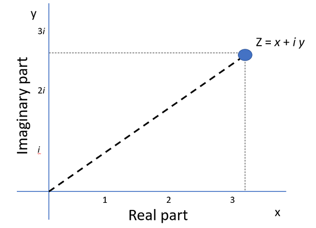
Every complex number x + yi can be graphed as an ordered pair (x, y).
The complex number i is the point (1, 0) on the plane and the real number 1 is represented by the point (0, 1). The following graph shows three numbers: 1 (green), i (orange), and 2 + 3i (blue):
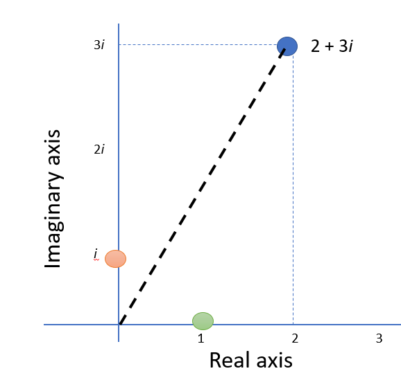
The equation z = 2 + 3i, graphed in this way, is called the rectangular form of the number z; the dashed lines fill in the shape of the rectangle on the above graph.
Notation
- Complex numbers and the complex plane are usually denoted with a doublestruck C (ℂ).
- Real variables: x, y or sometimes a, b.
- Complex variables: z, w
Complex Function
While a “regular” function has one or more real numbers, complex functions (also called complex-valued functions) are defined with one or more complex numbers. Complex numbers are made up of part real numbers and part imaginary numbers.
Complex functions are just functions that map from complex numbers to complex numbers. Since the complex values from their range and from their domain can both be separated into real and imaginary parts, we can split the complex function up into real and imaginary parts too.
![]()
Here x, y, and the functions u(x,y) and v(x,y) are all real-valued. We haven’t changed anything, but sometimes it is easier to understand the complex function f if we think of it as decomposed into these real-valued parts.
If a complex function is differentiable at every point of an open subset Ω of the complex plane we call it holomorphic on Ω Holomorphic functions are infinitely differentiable, and the study of them is a big part of complex analysis.
A More Formal Definition
In notation, we can say that a complex function f(z) contains complex variables where z ∈ ℂ. The doublestuck C (ℂ) is the set of complex numbers. Another way to say this is that a complex-valued function has a range entirely made up of complex numbers.
Note: Don’t confuse the “z” here with the z-axis. It has an entirely different meaning and, despite the complex numbers, is a two-dimensional problem.
The formal definition of a complex function isn’t that much different from the one involving real-numbered functions. The definition involves one-to-one mapping, which is the fundamental idea behind a function. For real-numbered functions, each input (x) gets mapped to exactly one output f(x). In the case of a complex function, each element of z (the input) gets mapped to exactly one complex-numbered output— f(z).
A Few Examples
For a complex function f(z) = u + iv, the function u(x, y) is the real-numbered part of f and v(x, y) is the imaginary part. With that out of the way, functions F(z) are written in the same way as you would write a real-valued function.
Some of the simpler complex functions don’t look much different from their real-numbered counterparts. For example, the constant function f(z) = c (where c is a constant that can be complex) or the absolute value function f(z) = |z|. The identity map looks very similar as well: f(z) = z.
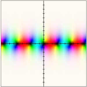
Graphing Complex Functions
Graphing a complex function is challenging because you need 4 dimensions: two for the domain and two for the range. That’s because instead of the usual “y” output, a complex function outputs another complex number. Several graphers are available online, including this one, which uses domain coloring to address the four-dimensional problem. The grapher will graph slowly, although you can make it go faster by increasing the accuracy.
References
Beck, M. et al. (2018). A First Course in Complex Analysis. Retrieved November 27, 2019 from: http://math.sfsu.edu/beck/papers/complexorth.pdf
Cain, George. Complex Analysis. Retrieved from https://people.math.gatech.edu/~cain/winter99/complex.html on August 11, 2019
Complex Functions and the Cauchy-Riemann Equations. Retrieved November 27, 2019 from: https://www.math.columbia.edu/~rf/complex2.pdf
Berg, Christian. Complex Analysis. Retrieved from http://web.math.ku.dk/noter/filer/koman-12.pdf on August 11, 2019.
Hargittai, Istvan (Ed.). (1994). Fivefold Symmetry. World Publishing.
Joyce, D. Dave’s Short Course on Complex Numbers. Retrieved December 9, 2019 from: https://www2.clarku.edu/faculty/djoyce/complex/plane.html
Maseres, Francis. (1758). Dissertation on the Use of the Negative Sign in Algebra. Retrieved December 31, 2015 from: http://lhldigital.lindahall.org/cdm/ref/collection/math/id/4015
The Story of Mathematics. (2010).16th Century Mathematics — Tartaglia, Cardano & Ferrari. Retrieved December 31, 2015.
Waldemar Dos Passos. (2011). Numerical Methods, Algorithms, and Tools in C#. CRC Press.
Laurent Series
A Laurent series is a way to represent a complex function f(z) as a complex power series with negative powers.
This generalization of the Taylor series has two major advantages:
- The series can include both positive and negative powers,
- It can be expanded around singularities to analyze functions in neighborhoods around those singularities.
Watch the video for a short introduction or read on below:
Why These Series Are Useful
When these series represent deleted neighborhoods around a singularity, they can be useful for identifying essential discontinuities. Specifically, a singularity is essential if the principal part of the Laurent series has infinitely many nonzero terms (Kramer, n.d.).
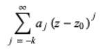
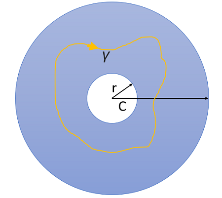
A punctured disk (a disc with a pinprick in the center), 0 < |z – z0 | < can also be written in terms of a Laurent series. Let’s say the series is:
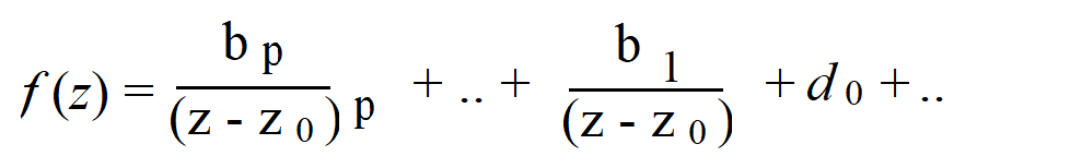
Then we can say that z0 is a pole of order p.
Use of Laurent Series vs Taylor Series
A Taylor series expansion can only express a function as a series with non-negative powers, so the Laurent series becomes very useful when you can’t use a Taylor series. Another way to think of a Laurent series is that—unlike the Taylor series—it allows for the existence of poles.
Formal Definition
If a function f(z) is analytic on the annulus:
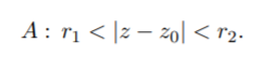
The function can be represented by (Orloff, 2020):
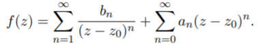
The principal part of the series is any term with negative powers of z – z0. This part can include a finite number or terms, or an infinite number of terms (Stephenson & Radmore, 1990).
The Laurent series is a natural generalization of the Taylor series when the expansion center is a pole (isolated singularity) instead of a non-singular point (Needham, 1998); The neighborhood around the pole can be represented by the series.
References
Kramer, P. L.S. Examples. Retrieved August 22, 2020 from: http://eaton.math.rpi.edu/faculty/Kramer/CA13/canotes111113.pdf
Needham, T. (1998). Visual Complex Analysis. Clarendon Press.
Orloff, J. (2020). Topic 7 Notes. Retrieved August 22, 2020 from: https://math.mit.edu/~jorloff/18.04/notes/topic7.pdf
Stephenson, G. & Radmore, P. (1990). Advanced Methods for Engineering and Science. Cambridge University Press.
Complex Analysis III. Laurent Series and Singularities. Retrieved August 22, 2020 from: http://howellkb.uah.edu/MathPhysicsText/Complex_Variables/Laurent.pdf