Covariance in Statistics: What is it? Example

Covariance: contents:

1. Definition & Formula
2. Example
3. Covariance vs. variance
4. Covariance vs. Correlation
5. Covariance in Excel

Definition & Formula

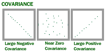
Covariance measures joint variability — the extent of variation between two random variables. It is similar to variance, but while variance quantifies the variability of a single variable, covariance quantifies how two variables vary together. The measure can be positive, negative, or zero [1]:

• • Positive covariance = an overall tendency for variables to move together. Data points will trend upwards on a graph.

• • Negative covariance = a overall tendency that when one variable increases, so does the other. Data points will trend downward on a graph.

A high covariance indicates a strong relationship between the variables, while a low value suggests a weak relationship. However, unlike the correlation coefficient — which ranges from 0 to 1 — covariance has no limitations on its values, which can make it challenging to interpret.

Covariance is defined for each pair of variables in the probability density function (pdf). Thus, there would be three covariances for a trivariate distribution P(x, y, z): cov(x, y), cov(x, z) and cov(y, z) [2]. The covariance of a random variable and itself is just its variance [3].

The Covariance Formula

The formula is: Cov(X,Y) = Σ E((X – μ) E(Y – ν)) / n-1 where:

• X is a random variable
• E(X) = μ is the expected value (the mean) of the random variable X and
• E(Y) = ν is the expected value (the mean) of the random variable Y
• n = the number of items in the data set.
• Σ summation notation.

Back to top

Examples

Example 1: Calculate covariance for the following data set: x: 2.1, 2.5, 3.6, 4.0 (mean = 3.1) y: 8, 10, 12, 14 (mean = 11)

Substitute the values into the formula and solve:

• Cov(X,Y) = ΣE((X-μ)(Y-ν)) / n-1 =
• (2.1-3.1)(8-11)+(2.5-3.1)(10-11)+(3.6-3.1)(12-11)+(4.0-3.1)(14-11) /(4-1) =
• (-1)(-3) + (-0.6)(-1)+(.5)(1)+(0.9)(3) / 3 =
• 3 + 0.6 + .5 + 2.7 / 3 =
• 6.8/3 =
• 2.267

The result is positive, meaning that the variables are positively related.

Note on dividing by n or n-1: When dealing with samples, there are n-1 terms that have the freedom to vary (see: Degrees of Freedom). We only know sample means for both variables, so we use n – 1 to make the estimator unbiased. for very large samples, n and n – 1 would be roughly equal (i.e., for very large samples, we would approach the population mean).

Example 2:  Suppose we have the following dataset:

Value	X	Y
1	2.1	8
2	2.5	10
3	3.6	12
4	4.0	14

1. Find the means of X and Y:
   • Mean of X = (2.1 + 2.5 + 3.6 + 4.0) / 4 = 3.05
   • Mean of Y = (8 + 10 + 12 + 14)/4 = 11.
2. Subtract each mean from its corresponding term, then multiply:
   • = (x₁ ​− x̄) * (y₁​ − ȳ​) + (x₂ ​− x̄) * (y₂ ​− ȳ​) + (x₃ ​− x̄) * (y₃ ​− ȳ​) + (x₄ ​− x̄)(y₄ ​− ȳ​)
   • = (2.1 – 3.05) * (8 – 11) + (2.5 – 3.05) * (10 – 11) + (3.6 – 3.05) * (12 – 11) + (4.0 – 3.05) * (14 – 11) = 6.8.
3. Divide by the number of values in the sample – 1:
   • s_xy = 6.8/ 3 = 2.27.

A positive covariance of 2.27 suggests a positive trend, where the two variables vary together.

Back to top

Covariance vs. variance

Covariance is associated with variance, a statistical measure of point dispersion in a data set. Both variance and covariance quantify the distribution of data points around a calculated mean. However, variance assesses how data spread is spread about the mean along a single axis, whereas covariance explores the directional relationship between two variables.

Take, for instance, a case where we have two variables: height and weight. The variance of height would indicate the extent to which the heights of individuals in our dataset differ from the average height. Similarly, the covariance of height and weight would show how the heights and weights of individuals in our dataset co-vary.

Covariance vs correlation / Problems with interpretation

Corr(X,Y) = Cov(X, Y) /  σ_Xσ_Y

There are many advantages of using a correlation coefficient instead of covariance when assessing the strengths of relationships:

• While Cov. has no limitations on its values, correlation is restricted to the range of -1 to +1.
• Due to its numerical constraints, correlation is more suitable for determining the strength of the relationship between the two variables: a correlation coefficient of 0 indicates no relationship, a correlation coefficient of 1 or -1 indicates a perfect relationship.
• Correlation is unitless, whereas covariance always carries units. This is because the correlation coefficient is standardized, which removes units of measurement from calculations. This makes it easier to interpret the correlation coefficient.
• Correlation is unaffected by changes in the center of a distribution (e.g., mean) or scale of the variables. This is because the correlation coefficient is calculated using deviations from the mean of the variables.

A large covariance can mean a strong relationship between variables. However, you can’t compare variances over data sets with different scales (like pounds and inches). A weak covariance in one data set may be a strong one in a different data set with different scales.

The main problem with interpretation is that the wide range of results that it takes on makes it hard to interpret. For example, your data set could return a value of 3, or 3,000. This wide range of values is cause by a simple fact; The larger the X and Y values, the larger the covariance. A value of 300 tells us that the variables are correlated, but unlike the correlation coefficient, that number doesn’t tell us exactly how strong that relationship is.

The problem can be fixed by dividing the covariance by the standard deviation to get the correlation coefficient. Corr(X,Y) = Cov(X,Y) / σ_Xσ_Y

The Correlation Coefficient has several advantages over covariance for determining strengths of relationships:

• Covariance can take on practically any number while a correlation is limited: -1 to +1.
• Because of it’s numerical limitations, correlation is more useful for determining how strong the relationship is between the two variables.
• Correlation does not have units. Covariance always has units
• Correlation isn’t affected by changes in the center (i.e. mean) or scale of the variables

Back to top

Calculate covariance in Excel

Covariance gives you a positive number if the variables are positively related. You’ll get a negative number if they are negatively related. A high covariance basically indicates there is a strong relationship between the variables. A low value means there is a weak relationship.

Covariance in Excel: steps

1. Enter your data into two columns in Excel. For example, type your X values into column A and your Y values into column B.
2. Click the “Data” tab and then click “Data analysis.” The Data Analysis window will open.
3. Choose “Covariance” and then click “OK.”
4. Click “Input Range” and then select all of your data. Include column headers if you have them.
5. Click the “Labels in First Row” check box if you have included column headers in your data selection.
6. Select “Output Range” and then select an area on the worksheet. A good place to select is an area just to the right of your data set.
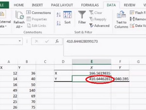
7. Click “OK.” The covariance will appear in the area you selected in Step 5. That’s it!

Tip: Run the correlation function in Excel after you run covariance in Excel 2013. Correlation will give you a value for the relationship. 1 is perfect correlation and 0 is no correlation. All you can really tell from covariance is if there is a positive or negative relationship.

Check out our YouTube channel for more Excel tips and help!

Back to top

References

1. Joyce, D. (2014). Cov. and Correlation Math 217 Probability and Statistics. Retrieved August 16, 2023 from: http://aleph0.clarku.edu/~djoyce/ma217/covar.pdf
2. Caltech. Statistics and the treatment of experimental data.
3. LECTURE NOTES 4 1

References

Dodge, Y. (2008). The Concise Encyclopedia of Statistics. Springer.
Everitt, B. S.; Skrondal, A. (2010), The Cambridge Dictionary of Statistics, Cambridge University Press.
Gonick, L. (1993). The Cartoon Guide to Statistics. HarperPerennial.