Contents:
Probability Integral
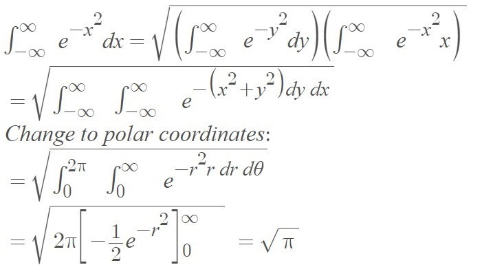
The probability integral (also called the Gaussian Integral) is the integral of the one-dimensional Gaussian (or normal distribution) over (-∞,∞).
It can be calculated by combining two Gaussians then changing to polar coordinates:

Historically, the integral was calculated with tables but now they are usually calculated with computer software.
Probability integral of the normal distribution
This term refers to the integral of the normal distribution, where the total area under the curve is normalized to 1 (for example, see [1]):

Probability Integral Transform
Also called the CDF transform, this is a way to transform a cumulative distribution function (CDF) in terms of one variable into another CDF in terms of a different variable.
More formally, it states that given a continuous random variable X with CDF FX, then the random variable Y = FX(X) will be uniformly distributed on the closed interval [0, 1].
The transformation X = F-1X(U) is called the inverse probability integral transformation [2].
The probability integral transform is often used to generate random variables that follow a specified probability distribution. For example, let’s say a researcher wants to estimate failure time for an airplane’s circuit component. While uniformly distributed variables are relatively easy to generate, the researcher wants to generate variables from an exponential distribution, because they think that the component’s failure time is exponentially distributed with parameter λ with probability distribution then Y = e−λX [3].
The probability integral transform tell us that if X has an Exponential (&malbda;) distribution, then Y = e−λX has a Uniform [0, 1] distribution.
References
[1] Lecture 3: Gaussian probability distribution.
[2] Kay, S. (2006). Intuitive probability and random processes using MATLAB. Springer US.
[3] Kapadia et. al. (2005). Mathematical statistics with applications. Taylor & Francis.