Contents:
What is an Ordinary Integral?
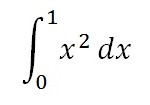
An ordinary integral is another name for the plain old single integral, consisting of:
- A function to be integrated (an integrand) over the real (numbers) line,
- One variable to integrate over (e.g. x or y),
- A region of space to integrate over (a domain of integration).
Another way to define an ordinary integral: It’s the only one where you can use the fundamental theorem of calculus to find a solution. With other types, you can’t directly use the theorem; You have to manipulate the integral in some way first.
Comparison of Ordinary Integral to Other Integrals
Although it’s usually called just an “integral” in introductory calculus, it’s referred to as “ordinary” in higher calculus texts to set it apart from other integrals, like:
- Line integrals (generalized ordinary integrals that work along curves),
- Product integrals (which have multiplication instead of summation),
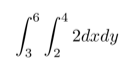
- Double integrals (a stack of two single integrals). With an ordinary (single) integral, you can use the fundamental theorem of calculus to integrate over a region. A 2-dimensional double integral has to be broken apart into two 1-dimensional ordinary integrals before it can be evaluated (Goetz, 2020).
Why are they called “Ordinary”?
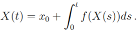
Ordinary integrals are called ordinary because they are equal to ordinary differential equations (Hall, 2012). For example, the following ordinary differential equation, with initial condition X(0) = x0
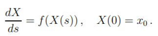
is equivalent to finding a solution to the following ordinary integral (Papaspiliopoulos, 2007):
What is a Multiple Integral?
Multiple integrals are definite integrals and are an extension of the ordinary (single) integral, which finds an area below a curve. Usually, the focus is on double integrals, which find the area of a region in a plane, and triple integrals which find volumes.
Multiple integrals arise in many areas of physical science, especially in mechanics to find volumes, masses, and moments of inertia.
Types of Multiple Integrals
- Double Integrals
- Triple Integrals
- Multiple Integrals for Higher Dimensions
1. Double Integrals
 Double integrals allow you to find the volume for a two-dimensional area or surface. General steps to solving:
- Evaluate the inner integral,
- Substitute the result into the equation,
- Solve the outer integral.
For a step by step example, see: Double Integral Worked Example.
2. Triple Integrals
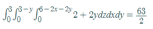
Triple integrals extend integration to find 3D volumes or mass, when the volume has variable density. For a worked example, see: Center of mass with triple integrals.
3. Multiple Integrals for Higher Dimensions
It’s theoretically possible to have a multiple integral for any number of dimensions. For example, quadruple integrals find hypervolumes: the volume of objects in four-dimensional space.
Let’s say we had a 4-D box in a space with coordinates (x, y, z, w). the quadruple integral could be defined in the same way as integrals in lower dimensions are defined: as limits of Riemann sums:
- Subdivide the box into i j k l equal-sized boxes:
- i boxes in the x direction,
- j boxes in the y direction,
- k boxes in the z direction,
- l boxes in the w direction.
- Sample one point in each box, multiplying f at the point * the volume of the box,
- Sum up over all boxes.
The quadruple integral is the limit of i j k l as they go to infinity [1].
Integrals in higher dimensions are rarely seen as they have little practical use and are challenging to calculate. For example the stream depletion rate (in hydrology) can be expressed as a quintuple integral, but the solution requires less computational effort when computing four of the integrals analytically [2].
References
[1] Rowan, J. (2018). Math 53 Summer 2018 Homework Assignment 20: Solutions to selected problems. Retrieved May 5, 2021 from: https://math.berkeley.edu/~jrowan/53Summer18/MATH53Su18ROWAN-ASSIGNMENT20SOLNS.pdf
[2] Maroney, C. & Rehmann, C. (2017). Stream depletion rate for a radial collector well in an unconfined aquifer near a fully penetrating river. Journal of Hydrology, Volume 547, April, Pages 732-741
References
Goetz, P. (2020). LM15-2-2. Retrieved September 1, 2020 from: https://web.ma.utexas.edu/users/m408s/m408d/current/LM15-2-2-pgoetz.html
Hall, W. (2012). The Boundary Element Method. Springer Netherlands.
Papaspiliopoulos, A. (2007). An introduction to modelling and likelihood inference with stochastic differential equations. Retrieved September 1, 2020 from: http://84.89.132.1/~omiros/course_notes.pdf