Numerical Differentiation

Many known functions have exact derivatives. For example, the derivative of the natural logarithm, ln(x), is 1/x. Other functions involving discrete data points don’t have known derivatives, so they must be approximated using numerical differentiation. The technique is also used when analytic differentiation results in an overly complicated and cumbersome expression (Bhat & Chakraverty, 2004).

Interpolation as a Numerical Differentiation Method

One of the easiest ways to approximate a derivative for a set of discrete points is to create an interpolation Function, which gives an estimated continuous function for the data. Once you have the estimated function (for example a polynomial function), you can then use known derivatives.

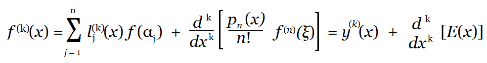
If the function is given as a table of values, a similar approach is to differentiate the Lagrange interpolation formula to get (Ralston & Rabinowitz, 2001):
numerical differentiation

Numerical Differentiation using Differences

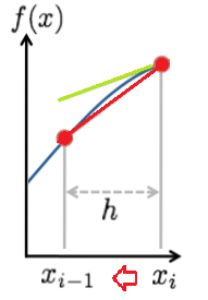
Differences are a set of tools for estimating the derivative using a set range of x-values. The basic idea is that the algorithms “move” the points so that they get closer and closer together, to look like a tangent line. Exactly how the points are moved (for example, forwards or backwards) gives rise to three common algorithms: backward differencing, forward differencing, and central differencing.

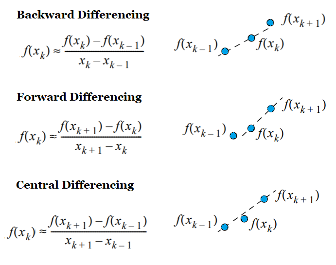
Forward differencing (a one-sided differencing algorithm) is based on values of the function at points x and x + h.
Backward differencing (also one-sided)is based on values at x and x – h.
Central (or centered) differencing is based on function values at f(x – h) and f(x + h).

While all three formulas can approximate a derivative at point x, the central difference is the most accurate (Lehigh, 2020).

Let’s say you have a table with the following values, and you want to approximate the derivative at x = 0.5 using the central difference.

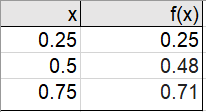
Using the formula from above, you would get:
F′(x) = (0.71 – 0.25) / 0.25 = 0.92.

Backward Differencing

Backward differencing is a way to estimate a derivative with a range of x-values. The algorithm “moves” the points closer and closer together until they resemble a tangent line.

Backward Differencing Formula

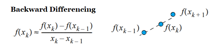
If you’ve calculated slopes before, the formula might look familiar: it’s a variation on the theme. There are four parts to the formula:

x_k: The x-value you’re estimating at.
f(x_k): The function value at x_k.
x_k-1: The x-value, less the step size. For example, if you’re estimating at x = 2 with a step size of 1, then x_k-1 is 2 -1 = 1.
f(x_k-1): The function value at x_k-1.

Example question: Approximate the derivative of f(x) = x² + 2x at x = 3 using backward differencing with a step size of 1.

Step 1: Identify x_k. This is given in the question as x = 3.

Step 2: Calculate f(x_k), the function value at the given point. For this example, that’s at x = 3. Inserting that value into the formula we’re given in the question: (f(x) = x² + 2x ), we get:
f(3) = 3² + 2(3) = 15

Step 3: Identify x_k-1. This your x-value from Step 1, minus 1:
3 – 1 = 2.

Step 4: Find f(x_k-1), the function value one step behind. We’re given that the step size is 1 in the example problem, so we’re calculating the value at x = 2:
f(2) = 2² + 2(2) = 8

Step 5: Insert your values into the formula and solve:

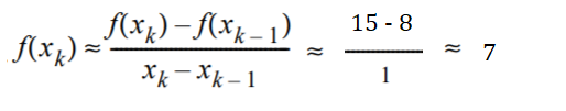
Other Types of Differencing

Other types of differencing are forward differencing, and central differencing.

Forward differencing: When h (the distance between the two points) is greater than zero (i.e. h > 0).
Backward differencing: When h < 0.
Central differencing: An average of the two methods (using three points).

graph backwards difference — You have to use backwards differences at the right endpoint of a function (at x_i).

For a given number of points, central differencing is more accurate. However, you can’t use central differencing at the left and right endpoints because there are no points further to the left or right with which to take an average. These methods come in useful when you have no data from the past or in the future beyond certain points. At these points you have to use forward differencing (left endpoint) and backwards differencing (right endpoint).

References

Andasari, V. (2020). Numerical Differentiation. Retrieved September 21, 2020 from: http://people.bu.edu/andasari/courses/Fall2015/LectureNotes/Lecture7_24Sept2015.pdf
Bhat, R. & Chakraverty, S. (2004). Numerical Analysis in Engineering. Alpha Science International.
Hoffman, J. & Frankel, S. (2001). Numerical Methods for Engineers and Scientists, Second Edition. Taylor & Francis.
Kutz, J. (2013). Data-Driven Modeling & Scientific Computation. Methods for Complex Systems & Big Data. OUP Oxford.
Lehigh University (2020). Numerical Differentiation. Retrieved September 6, 2020 from: https://www.lehigh.edu/~ineng2/clipper/notes/NumDif.htm
Levy, D. Numerical Differentiation. Retrieved September 6, 2020 from: http://www2.math.umd.edu/~dlevy/classes/amsc466/lecture-notes/differentiation-chap.pdf
Ralston, A. & Rabinowitz, P. (2001). A First Course in Numerical Analysis. Dover Publications.
MIT: Finite Difference Approximations.