Statistics Definitions > Multicollinearity
- What is Multicollinearity?
- What Causes Multicollinearity?
- What Happens to Analyses
- Detecting Multicollinearity
- Fixing Detected Multicollinearity
What is Multicollinearity?
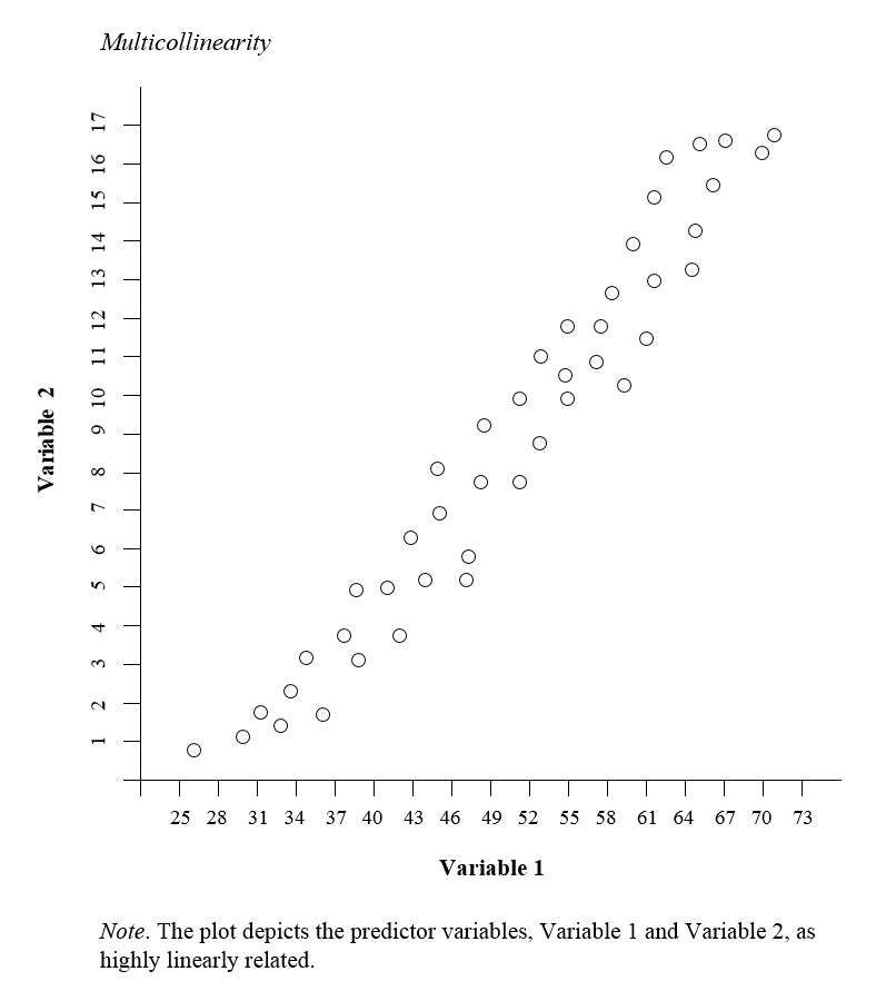
Multicollinearity occurs when two or more predictor variables in a regression model are highly correlated with each other. In other words, one predictor variable can be used to predict another with a considerable degree of accuracy. This creates redundant information, skewing regression analysis results.
Examples of multicollinear predictors (also called correlated predictor variables) are:
- Number of rooms and a house’s square footage.
- A person’s height and weight,
- Age and sales price of a car,
- Engine size and vehicle weight,
- Years of education and annual income.
What Causes Multicollinearity?
The two types are:
- Data-based multicollinearity: caused by poorly designed experiments, data that is 100% observational, or data collection methods that cannot be manipulated. In some cases, variables may be highly correlated (usually due to collecting data from purely observational studies) and there is no error on the researcher’s part. For this reason, you should conduct experiments whenever possible, setting the level of the predictor variables in advance.
- Structural multicollinearity: caused by you, the researcher, creating new predictor variables.
Causes for multicollinearity can also include:
-
- Insufficient data. In some cases, collecting more data can resolve the issue.
- Dummy variables may be incorrectly used. For example, the researcher may fail to exclude one category, or add a dummy variable for every category (e.g. spring, summer, autumn, winter).
- Including a variable in the regression that is actually a combination of two other variables. For example, including “total investment income” when total investment income = income from stocks and bonds + income from savings interest.
- Including two identical (or almost identical) variables. For example, weight in pounds and weight in kilos, or investment income and savings/bond income.
What Happens to Analyses
It’s more common for multicollinearity to rear its ugly head in observational studies; it’s less common with experimental data. When the condition is present, it can result in unstable and unreliable regression estimates.
Detecting Multicollinearity
One relatively easy way to detect multicollinearity is to calculate correlation coefficients for all pairs of predictor variables. If the correlation coefficient, r, is exactly +1 or -1, this is called perfect multicollinearity. If r is close to or exactly -1 or +1, one of the variables should be removed from the model if at all possible
Other methods include correlation matrices, variance inflation factors, and tolerance levels.
1. Correlation Matrices
A correlation matrix displays the correlation coefficients between all pairs of predictor variables in your dataset. These coefficients indicate the strength and direction of the linear relationship between variables.
- Generate the Correlation Matrix: Create a matrix to show correlations between predictor variables. Most statistical software can create correlation matrices, although it’s possible to create on on a spreadsheet.
- Identify High Correlations: Look for pairs of variables with high correlation coefficients (above 0.8 or 0.9 or below -0.8 or -0.9). These indicate strong relationships.
High correlation between two variables suggests that the variables may be giving redundant information. This is an indication of multicollinearity between those predictors.
A limitation is that a correlation matrix can only detect Pairwise Relationships. Therefore, it may miss more complex multicollinearity involving multiple variables simultaneously.
2. Variance Inflation Factors (VIFs)
The Variance Inflation Factor (VIF) measures how much the variance of a regression coefficient is increased due to multicollinearity. It assesses the extent to which a predictor variable can be explained by other predictor variables in the model.
How to Use VIFs:
- Compute VIFs for Each Predictor Variable:
- Statistical software can calculate VIF values for all predictors in your regression model.
- Assess the VIF Values:
- VIF = 1:
- Indicates no correlation with other predictors.
- VIF between 1 and 5:
- Suggests moderate correlation but is generally acceptable.
- VIF above 5 (or 10):
- Indicates a high level of multicollinearity that may need to be addressed.
- VIF = 1:
Advantages:
- Considers Multivariate Relationships:
- VIF accounts for the combined effect of all other predictors on a given predictor, not just pairwise correlations.
3. Tolerance Levels
Tolerance is closely related to VIF and represents the proportion of a predictor’s variance that is not explained by other predictors in the model.
How to Use Tolerance Levels:
- Calculate Tolerance for Each Predictor:
- Tolerance is often computed automatically by statistical software alongside VIF.
- Assess Tolerance Values:
- Tolerance Close to 1:
- Indicates low multicollinearity; most of the variance is unique to that predictor.
- Tolerance Near 0:
- Indicates high multicollinearity; the predictor shares a lot of variance with other predictors.
- Tolerance Close to 1:
Advantages:
- Complementary to VIF:
- Since tolerance is the inverse of VIF, it provides the same information in a different format, which some find more intuitive.