Statistics Definitions > Factor Analysis
Contents:
- What is Factor Analysis?
- Factor Loadings
- Multiple Factor Analysis
- Confirmatory Factor Analysis
- Exploratory Factor Analysis
- What is Generalized Procrustes Analysis (GPA)
- What are Latent Variables?
- What are Manifest Variables?
1. What is Factor Analysis?
Factor analysis is a way to take a mass of data and shrinking it to a smaller data set that is more manageable and more understandable. It’s a way to find hidden patterns, show how those patterns overlap and show what characteristics are seen in multiple patterns. It is also used to create a set of variables for similar items in the set (these sets of variables are called dimensions). It can be a very useful tool for complex sets of data involving psychological studies, socioeconomic status and other involved concepts.
A “factor” is a set of observed variables that have similar response patterns; They are associated with a hidden variable (called a confounding variable) that isn’t directly measured. Factors are listed according to factor loadings, or how much variation in the data they can explain.
The two types: exploratory and confirmatory.
- Exploratory factor analysis is if you don’t have any idea about what structure your data is or how many dimensions are in a set of variables.
- Confirmatory Factor Analysis is used for verification as long as you have a specific idea about what structure your data is or how many dimensions are in a set of variables.
2. Factor Loadings
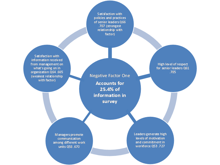
Not all factors are created equal; some factors have more weight than others. In a simple example, imagine your bank conducts a phone survey for customer satisfaction and the results show the following factor loadings:
| Variable | Factor 1 | Factor 2 | Factor 3 | Question 1 | 0.885 | 0.121 | -0.033 |
|---|---|---|---|
| Question 2 | 0.829 | 0.078 | 0.157 |
| Question 3 | 0.777 | 0.190 | 0.540 |
The factors that affect the question the most (and therefore have the highest factor loadings) are bolded. Factor loadings are similar to correlation coefficients in that they can vary from -1 to 1. The closer factors are to -1 or 1, the more they affect the variable. A factor loading of zero would indicate no effect.
3. Multiple Factor Analysis
This subset of Factor Analysis is used when your variables are structured in variable groups. For example, you might have a student health questionnaire with several items like sleep patterns, addictions, psychological health, or learning disabilities.
The two steps performed in Multiple Factor Analysis are:
- Principal Component Analysis is performed on each set of data. This gives an eigenvalue, which is used to normalize the data sets.
- The new data sets are merged into a unique matrix and a second, global PCA is performed.
Performing Factor Analysis
Factor Analysis is an extremely complex mathematical procedure and is performed with software.
- Instructions for Stata can be found here.
- Minitab instructions are here.
- For SPSS, FactorAnalysisHowTo.
The Kaiser-Meyer-Olkin test checks to see if your data is suitable for FA.
Back to Top
4. What is Confirmatory Factor Analysis?
Confirmatory Factor Analysis allows you to figure out if a relationship between a set of observed variables (also known as manifest variables) and their underlying constructs exists. It is similar to Exploratory Factor Analysis. The main difference between the two is:
- If you want to explore patterns, use EFA.
- If you want to perform hypothesis testing, use CFA.
EFA provides information about the optimal number of factors required to represent the data set. With Confirmatory Factor Analysis you can specify the number of factors required. For example, CFA can answer questions like “Does my ten question survey accurately measure one specific factor?”. Although it is technically applicable to any discipline, it is typically used in the social sciences.
Implementing Confirmatory Factor Analysis
Diane Suhr, PhD, on the SAS website, suggests the following steps:
- Perform a literature review to help you choose an appropriate model. For example, you might choose a diagram or equations.
- Determine if unique value are possible for the population parameter estimation.
- Collect your data.
- Perform initial data analysis to check for issues like missing data, collinearity or outliers.
- Estimate the population parameters.
- Determine if the model you chose is working. If the model is unacceptable, consider performing Explanatory Factor Analysis.
- Interpret your results.
According to IBM, EFA has overtaken CFA as a means of Factor Analysis. “The predominant CFA approach today is to consider CFA as a special case of structural equation modeling (SEM). You specify factor loadings as a set of regression statements from the factor to the observed variables.” With EFA, it’s possible to specify a few factors and a particular rotation; you can then compare your results to see if they fit your model.
Performing CFA

Software is usually required to perform confirmatory factor analysis. SAS can be used to perform CFA. At the time of writing, SPSS is limited to EFA only.
- SAS CFA procedure.
- AMOS instructions (download document from East Carolina University).
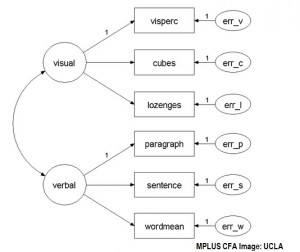
- AMOS, LISREL, MPLUS procedures.
5. What is Exploratory Factor Analysis?
Exploratory Factor Analysis(EFA) is used to find the underlying structure of a large set of variables. It reduces data to a much smaller set of summary variables.
EFA is almost identical to Confirmatory Factor Analysis(CFA). Both techniques can (perhaps surprisingly) be used to confirm or explore. Similarities are:
- Assess the internal reliability of a measure.
- Examine factors or theoretical constructs represented by item sets. They assume the factors aren’t correlated.
- Investigate quality for individual items.
There are, however, some differences, mostly concerning how factors are treated/used. EFA is basically a data-driven approach, allowing all items to load on all factors, while with CFA you must specify which factors to load. EFA is a good choice if you don’t have any idea about what common factors might exists. EFA can generate a large number of possible models for your data, something that may not be possible if a researcher has to specify factors. If you do have an idea about what the models look like, and you want to test your hypotheses about the data structure, CFA is a better approach.
6. What is Generalized Procrustes Analysis (GPA)?
Procrustes analysis is a way to compare two sets of configurations, or shapes. Originally developed to match two solutions from Factor Analysis, the technique was extended to Generalized Procrustes Analysis so that more than two shapes could be compared. The shapes are aligned to a target shape or to each other.
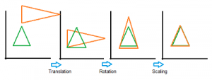
GPA uses geometric transformations (i.e. isotropic rescaling, reflection, rotation, or translation) of matrices to compare the sets of data. The following image shows a series of transformations onto a green target triangle.

The consensus matrix is (as the name suggests), the result of the averages of all of the input matrices. The matrices formed during the Generalized Procrustes Analysis process can be input into Principal Components Analysis and projected onto two-dimensional space for easily understood results.
Use in Sensory Profiling
Generalized Procrustes Analysis a way to find an underlying structure in sensory profiling, which falls into two categories: conventional profiling and free-choice profiling.
With conventional profiling, a fixed set of descriptive terms is provided for the assessors. The assessors are usually highly trained individuals. For example, you could ask three experts their opinions on the body, scent and taste of four brands of wine. The fixed descriptions might include crisp, angular, and buttery. The results can be averaged, so it’s possible to use Factor Analysis or Principal Component Analysis—as well as GPA—to analyze the test.
Free-choice profiling gives respondents the freedom to answer questions in their own descriptive terms. As there are no fixed terms to average, it’s not possible to use Factor Analysis or PCA. K-sets methods, like PCA, are used on this type of free-choice profiling.
The categories are the dimensions of Generalized Procrustes Analysis. Ideally, the number of dimensions is equal across the board (in this example, that would mean the expert gave a rating in all three areas). However, it is possible to run Generalized Procrustes Analysis using unequal dimensions.
Back to Top
7. What are Latent Variables?
 A latent variable or “hidden” variable is generally thought of as a variable that is not directly measurable or observable. For example, a person’s level of neurosis, conscientiousness or openness are all latent variables. Although you can’t see these underlying variables (they aren’t part of an experiment’s data set) they can cause effects in your experimental results. Latent variables are also known as:
- Constructs or Hypothetical Constructs.
- Factors.
- Hidden Variables.
- Hypothetical Variables.
- True scores.
- Unmeasured variables.
- Unobserved variables.
One of the earliest examples of a latent variable was published in 1904 when Spearman measured intelligence using factor analysis. A more precise definition of latent variables is sometimes used. For example, MacCallum & Austin(2000) describe these variables as “hypothetical constructs that cannot be directly measured.” They are hypothetical because they only exist in the minds of the researcher.
The Latent Variable in Statistical Modeling
Latent variables are sometimes used in statistical modeling techniques like Factor Analysis, where they can be inferred though modeling techniques. Latent variables are ever-present in nearly all regression analysis, because all additive error terms are not measurable (and are therefore latent).
Statistical modeling methods that are often used to identify latent variables include:
- EM Algorithms.
- Factor Analysis.
- Hidden Markov Models.
- Latent Semantic Analysis.
- Principal Component Analysis.
- Structural Equation Modeling.
A latent variable can also be present (and included in a model) when there is no goal of actually measuring it. Melanie Wall of Columbia University offers the following three examples of latent variables that are not intended to be measured:
- Unobserved heterogeneity (e.g. frailties in survival analysis, random effects in longitudinal data or clustered data)
- Missing data
- Counterfactuals or ’potential outcomes’
What are Manifest Variables?
Manifest variables (also called observable variables) can be measured or observed directly. They are the opposite of latent variables. For example, age and gender are observable variables. However, it’s rare that you can be 100% certain about a variable; Even “gender”, if observed, isn’t 100% certain, because people may lie on their form, disguise their real gender, or be a transgender person. Therefore, you should use latent variables whenever possible.
References
MacCallum RC, Austin JT. 2000. Applications of structural equation modeling in psychological research. Annu. Rev. Psychol. 51:
201–26
