Correlation coefficients are used to measure how strong a relationship is between two variables. There are several types of correlation coefficient, but the most popular is Pearson’s. Pearson’s correlation (also called Pearson’s R) is a correlation coefficient commonly used in linear regression. If you’re starting out in statistics, you’ll probably learn about Pearson’s R first. In fact, when anyone refers to the correlation coefficient, they are usually talking about Pearson’s.
Watch the video for an overview of the correlation coefficient, or read on below:
- What is a correlation coefficient?
- Correlation coefficient formulas
- What is Pearson Correlation? How to Calculate:
- Cramer’s V Correlation
- Where did the Correlation Coefficient Come From?
- Correlation Coefficient Hypothesis Test.
- Relationship to cosine
- More Articles / Correlation Coefficients
What is a correlation coefficient?
A correlation coefficient is a measure of the strength of a linear relationship between two variables. In general, correlation coefficient values range from -1 to 1:
- 1 = a strong positive linear relationship. This means that for every positive increase in one variable, there is a proportional positive increase in the other variable. For instance, belt sizes increase almost perfectly in correlation with waist size.
- -1 = a strong negative linear relationship. In other words, for every positive increase in one variable, there is a proportional negative decrease in the other variable. As an example, the amount of gas in a vehicle’s tank decreases almost perfectly in correlation with speed.
- 0 = no linear relationship between the variables.
The absolute value of the correlation coefficient represents the strength of the relationship. A larger absolute value indicates a stronger relationship. For instance, |-.75| = .75, has a stronger relationship than .65. A “meaningful” correlation depends on the discipline [1]. For example, in physics, a correlation coefficient should be between -0.95 and 0.95, while in the social sciences, results between -0.6 and 0.6 are meaningful.
The Pearson correlation coefficient (also known as Pearson’s r) and Spearman’s rank correlation are the most widely used correlation coefficients [2]. However, there are many others including intraclass correlation and Moran’s I. If you’re just beginning elementary statistics, you’ll most likely be using Pearson’s correlation. Important! Calculating any correlation coefficient will give you an answer, but it should only be used to measure linear relationships. The easiest way to find out if your data meets this requirement is to create a scatter plot of your data before making any calculation. If your data looks roughly like a straight line, you can use Pearson’s r. If it’s random, or follows any other shape (U-shaped, S-shaped etc.), you should not calculate the correlation coefficient.
Correlation Coefficient Formula: Definition
Correlation coefficient formulas are used to find how strong a relationship is between data. The formulas return a value between -1 and 1, where:
- 1 indicates a strong positive relationship.
- -1 indicates a strong negative relationship.
- A result of zero indicates no relationship at all.

Meaning
- A correlation coefficient of 1 means that for every positive increase in one variable, there is a positive increase of a fixed proportion in the other. For example, shoe sizes go up in (almost) perfect correlation with foot length.
- A correlation coefficient of -1 means that for every positive increase in one variable, there is a negative decrease of a fixed proportion in the other. For example, the amount of gas in a tank decreases in (almost) perfect correlation with speed.
- Zero means that for every increase, there isn’t a positive or negative increase. The two just aren’t related.
The absolute value of the correlation coefficient gives us the relationship strength. The larger the number, the stronger the relationship. For example, |-.75| = .75, which has a stronger relationship than .65.
Types of correlation coefficient formulas.
There are several types of correlation coefficient formulas. One of the most commonly used formulas is Pearson’s correlation coefficient formula. If you’re taking a basic stats class, this is the one you’ll probably use:

Two other formulas are commonly used: the sample correlation coefficient and the population correlation coefficient.
Sample correlation coefficient
![]()
Sx and sy are the sample standard deviations, and sxy is the sample covariance.
Population correlation coefficient
![]()
The population correlation coefficient uses σx and σy as the population standard deviations, and σxy as the population covariance.
What is Pearson Correlation?
Correlation between sets of data is a measure of how well they are related. The most common measure of correlation in stats is the Pearson Correlation. The full name is the Pearson Product Moment Correlation (PPMC). It shows the linear relationship between two sets of data. In simple terms, it answers the question, Can I draw a line graph to represent the data? Two letters are used to represent the Pearson correlation: Greek letter rho (ρ) for a population and the letter “r” for a sample.
Potential problems with Pearson correlation.
The PPMC is not able to tell the difference between dependent variables and independent variables. For example, if you are trying to find the correlation between a high calorie diet and diabetes, you might find a high correlation of .8. However, you could also get the same result with the variables switched around. In other words, you could say that diabetes causes a high calorie diet. That obviously makes no sense. Therefore, as a researcher you have to be aware of the data you are plugging in. In addition, the PPMC will not give you any information about the slope of the line; it only tells you whether there is a relationship.
Real Life Example: Pearson correlation is used in thousands of real life situations. For example, scientists in China wanted to know if there was a relationship between how weedy rice populations are different genetically. The goal was to find out the evolutionary potential of the rice. Pearson’s correlation between the two groups was analyzed. It showed a positive Pearson Product Moment correlation of between 0.783 and 0.895 for weedy rice populations. This figure is quite high, which suggested a fairly strong relationship.
If you’re interested in seeing more examples of PPMC, you can find several studies on the National Institute of Health’s Openi website, which shows result on studies as varied as breast cyst imaging to the role that carbohydrates play in weight loss. Back to Top
How to Find Pearson’s Correlation Coefficients
By Hand
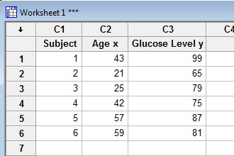
Example question: Find the value of the correlation coefficient from the following table: 143993257955787
| Subject | Age x | Glucose Level y |
|---|---|---|
| 2 | 21 | 65 |
| 4 | 42 | 75 |
| 6 | 59 | 81 |
Step 1: Make a chart. Use the given data, and add three more columns: xy, x2, and y2. 14399 32579 55787
| Subject | Age x | Glucose Level y | xy | x2 | y2 |
|---|---|---|---|---|---|
| 2 | 21 | 65 | |||
| 4 | 42 | 75 | |||
| 6 | 59 | 81 |
Step 2: Multiply x and y together to fill the xy column. For example, row 1 would be 43 × 99 = 4,257. 143994257 325791975 557874959
| Subject | Age x | Glucose Level y | xy | x2 | y2 |
|---|---|---|---|---|---|
| 2 | 21 | 65 | 1365 | ||
| 4 | 42 | 75 | 3150 | ||
| 6 | 59 | 81 | 4779 |
Step 3: Take the square of the numbers in the x column, and put the result in the x2 column. 1439942571849 325791975625 5578749593249
| Subject | Age x | Glucose Level y | xy | x2 | y2 |
|---|---|---|---|---|---|
| 2 | 21 | 65 | 1365 | 441 | |
| 4 | 42 | 75 | 3150 | 1764 | |
| 6 | 59 | 81 | 4779 | 3481 |
Step 4: Take the square of the numbers in the y column, and put the result in the y2 column. 14399425718499801325791975625624155787495932497569
| Subject | Age x | Glucose Level y | xy | x2 | y2 |
|---|---|---|---|---|---|
| 2 | 21 | 65 | 1365 | 441 | 4225 |
| 4 | 42 | 75 | 3150 | 1764 | 5625 |
| 6 | 59 | 81 | 4779 | 3481 | 6561 |
Step 5: Add up all of the numbers in the columns and put the result at the bottom of the column. The Greek letter sigma (Σ) is a short way of saying “sum of” or summation. 14399425718499801325791975625624155787495932497569
| Subject | Age x | Glucose Level y | xy | x2 | y2 |
|---|---|---|---|---|---|
| 2 | 21 | 65 | 1365 | 441 | 4225 |
| 4 | 42 | 75 | 3150 | 1764 | 5625 |
| 6 | 59 | 81 | 4779 | 3481 | 6561 |
| Σ | 247 | 486 | 20485 | 11409 | 40022 |
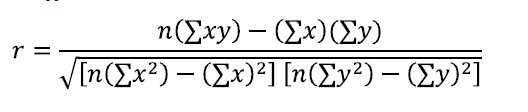
Step 6: Use the following correlation coefficient formula.  The answer is: 2868 / 5413.27 = 0.529809 From our table:
- Σx = 247
- Σy = 486
- Σxy = 20,485
- Σx2 = 11,409
- Σy2 = 40,022
- n is the sample size, in our case = 6
The correlation coefficient =
-
- 6(20,485) – (247 × 486) / [√[[6(11,409) – (2472)] × [6(40,022) – 4862]]]
= 0.5298 The range of the correlation coefficient is from -1 to 1. Our result is 0.5298 or 52.98%, which means the variables have a moderate positive correlation.
Correlation Formula: TI 83
If you’re taking AP Statistics, you won’t actually have to work the correlation formula by hand. You’ll use your graphing calculator. Here’s how to find r on a TI83.
- Type your data into a list and make a scatter plot to ensure your variables are roughly correlated. In other words, look for a straight line. Not sure how to do this? See: TI 83 Scatter plot.
- Press the STAT button.
- Scroll right to the CALC menu.
- Scroll down to 4:LinReg(ax+b), then press ENTER. The output will show “r” at the very bottom of the list.
Tip: If you don’t see r, turn Diagnostic ON, then perform the steps again.
How to Compute the Pearson Correlation Coefficient in Excel
Watch the video for an overview of the steps:

Can’t see the video? Click here to watch it on YouTube.
Step 1: Type your data into two columns in Excel. For example, type your “x” data into column A and your “y” data into column B.
Step 2: Select any empty cell.
Step 3: Click the function button on the ribbon. 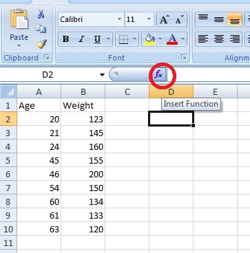
Step 4: Type “correlation” into the ‘Search for a function’ box. Step 5: Click “Go.” CORREL will be highlighted. 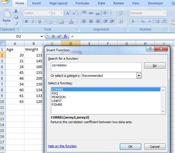
Step 6: Click “OK.”
Step 7: Type the location of your data into the “Array 1” and “Array 2” boxes. For this example, type “A2:A10” into the Array 1 box and then type “B2:B10” into the Array 2 box. 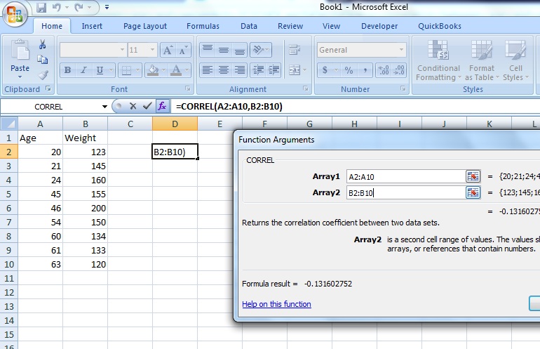
Step 8: Click “OK.”
The result will appear in the cell you selected in Step 2. For this particular data set, the correlation coefficient(r) is -0.1316. Caution: The results for this test can be misleading unless you have made a scatter plot first to ensure your data roughly fits a straight line. The correlation coefficient in Excel 2007 will always return a value, even if your data is something other than linear (i.e. the data fits an exponential model).
That’s it!
Correlation Coefficient SPSS: Overview.
Watch the video for an overview of how to do this, or read on below.

Can’t see the video? Click here to watch it on YouTube.
Step 1: Click “Analyze,” then click “Correlate,” then click “Bivariate.” The Bivariate Correlations window will appear. 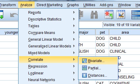 Step 2: Click one of the variables in the left-hand window of the Bivariate Correlations pop-up window. Then click the center arrow to move the variable to the “Variables:” window. Repeat this for a second variable.
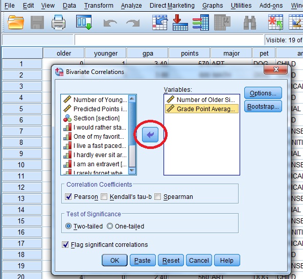
Step 3: Click the “Pearson” check box if it isn’t already checked. Then click either a “one-tailed” or “two-tailed” test radio button. If you aren’t sure if your test is one-tailed or two-tailed, see: Is it a a one-tailed test or two-tailed test?
Step 4: Click “OK” and read the results. Each box in the output gives you a correlation between two variables. For example, the PPMC for Number of older siblings and GPA is -.098, which means practically no correlation. You can find this information in two places in the output. Why? This cross-referencing columns and rows is very useful when you are comparing PPMCs for dozens of variables. 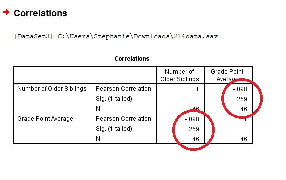 Tip #1: It’s always a good idea to make an SPSS scatter plot of your data set before you perform this test. That’s because SPSS will always give you some kind of answer and will assume that the data is linearly related. If you have data that might be better suited to another correlation (for example, exponentially related data) then SPSS will still run Pearson’s for you and you might get misleading results.
Tip #2: Click on the “Options” button in the Bivariate Correlations window if you want to include descriptive statistics like the mean and standard deviation.
Minitab
The Minitab correlation coefficient will return a value for r from -1 to 1. Example question: Find the Minitab correlation coefficient based on age vs. glucose level from the following table from a pre-diabetic study of 6 participants: 143993257955787
| Subject | Age x | Glucose Level y |
|---|---|---|
| 2 | 21 | 65 |
| 4 | 42 | 75 |
| 6 | 59 | 81 |
Step 1: Type your data into a Minitab worksheet. I entered this sample data into three columns.
Step 2: Click “Stat”, then click “Basic Statistics” and then click “Correlation.”
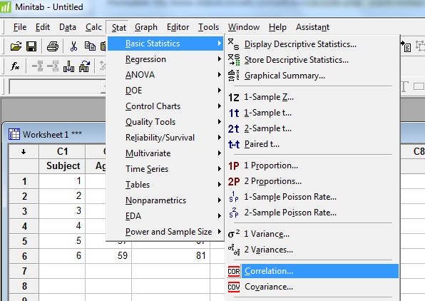
Step 3: Click a variable name in the left window and then click the “Select” button to move the variable name to the Variable box. For this example question, click “Age,” then click “Select,” then click “Glucose Level” then click “Select” to transfer both variables to the Variable window. 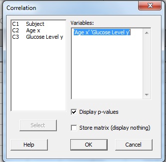 Step 4: (Optional) Check the “P-Value” box if you want to display a P-Value for r. Step 5: Click “OK”. The Minitab correlation coefficient will be displayed in the Session Window. If you don’t see the results, click “Window” and then click “Tile.” The Session window should appear.
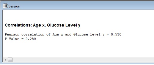
For this dataset:
- Value of r: 0.530
- P-Value: 0.280
That’s it!
Tip: Give your columns meaningful names (in the first row of the column, right under C1, C2 etc.). That way, when it comes to choosing variable names in Step 3, you’ll easily see what it is you are trying to choose. This becomes especially important when you have dozens of columns of variables in a data sheet!
Meaning of the Linear Correlation Coefficient.
Pearson’s Correlation Coefficient is a linear correlation coefficient that returns a value of between -1 and +1. A -1 means there is a strong negative correlation and +1 means that there is a strong positive correlation. A 0 means that there is no correlation (this is also called zero correlation). This can initially be a little hard to wrap your head around (who likes to deal with negative numbers?). The Political Science Department at Quinnipiac University posted this useful list of the meaning of Pearson’s Correlation coefficients. They note that these are “crude estimates” for interpreting strengths of correlations using Pearson’s Correlation:
| r value = | |
| +.70 or higher | Very strong positive relationship |
| +.40 to +.69 | Strong positive relationship |
| +.30 to +.39 | Moderate positive relationship |
| +.20 to +.29 | weak positive relationship |
| +.01 to +.19 | No or negligible relationship |
| 0 | No relationship [zero correlation] |
| -.01 to -.19 | No or negligible relationship |
| -.20 to -.29 | weak negative relationship |
| -.30 to -.39 | Moderate negative relationship |
| -.40 to -.69 | Strong negative relationship |
| -.70 or higher | Very strong negative relationship |
It may be helpful to see graphically what these correlations look like:
The images show that a strong negative correlation means that the graph has a downward slope from left to right: as the x-values increase, the y-values get smaller. A strong positive correlation means that the graph has an upward slope from left to right: as the x-values increase, the y-values get larger. Back to top.
Cramer’s V Correlation
Cramer’s V Correlation is similar to the Pearson Correlation coefficient. While the Pearson correlation is used to test the strength of linear relationships, Cramer’s V is used to calculate correlation in tables with more than 2 x 2 columns and rows. Cramer’s V correlation varies between 0 and 1. A value close to 0 means that there is very little association between the variables. A Cramer’s V of close to 1 indicates a very strong association.
| Cramer’s V | |
| .25 or higher | Very strong relationship |
| .15 to .25 | Strong relationship |
| .11 to .15 | Moderate relationship |
| .06 to .10 | weak relationship |
| .01 to .05 | No or negligible relationship |
Where did the Correlation Coefficient Come From?
A correlation coefficient gives you an idea of how well data fits a line or curve. Pearson wasn’t the original inventor of the term correlation but his use of it became one of the most popular ways to measure correlation. Francis Galton (who was also involved with the development of the interquartile range) was the first person to measure correlation, originally termed “co-relation,” which actually makes sense considering you’re studying the relationship between a couple of different variables. In Co-Relations and Their Measurement, he said
“The statures of kinsmen are co-related variables; thus, the stature of the father is correlated to that of the adult son,..and so on; but the index of co-relation … is different in the different cases.”
It’s worth noting though that Galton mentioned in his paper that he had borrowed the term from biology, where “Co-relation and correlation of structure” was being used but until the time of his paper it hadn’t been properly defined. In 1892, British statistician Francis Ysidro Edgeworth published a paper called “Correlated Averages,” Philosophical Magazine, 5th Series, 34, 190-204 where he used the term “Coefficient of Correlation.” It wasn’t until 1896 that British mathematician Karl Pearson used “Coefficient of Correlation” in two papers: Contributions to the Mathematical Theory of Evolution and Mathematical Contributions to the Theory of Evolution. III. Regression, Heredity and Panmixia. It was the second paper that introduced the Pearson product-moment correlation formula for estimating correlation.
Correlation Coefficient Hypothesis Test
If you can read a table — you can test for correlation coefficient. Note that correlations should only be calculated for an entire range of data. If you restrict the range, r will be weakened. Sample problem: test the significance of the correlation coefficient r = 0.565 using the critical values for PPMC table. Test at α = 0.01 for a sample size of 9.
Step 1: Subtract two from the sample size to get df, degrees of freedom. 9 – 7 = 2
Step 2: Look the values up in the PPMC Table. With df = 7 and α = 0.01, the table value is = 0.798
Step 3: Draw a graph, so you can more easily see the relationship. 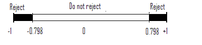 r = 0.565 does not fall into the rejection region (above 0.798), so there isn’t enough evidence to state a strong linear relationship exists in the data.
Relationship to cosine
It’s rare to use trigonometry in statistics (you’ll never need to find the derivative of tan(x) for example!), but the relationship between correlation and cosine is an exception. Correlation can be expressed in terms of angles:
- Positive correlation = acute angle <45°,
- Negative correlation = obtuse angle >45°,
- Uncorrelated = orthogonal (right angle).
More specifically, correlation is the cosine of an angle between two vectors defined as follows [3]:
If X, Y are two random variables with zero mean, then the covariance Cov[XY] = E[X · Y] is the dot product of X and Y. The standard deviation of X is the length of X.
Related Articles / More Correlation Coefficients
Other similar formulas you might come across that involve correlation (click for article):
- Concordance Correlation coefficient. Lin’s concordance correlation coefficient measures the extent to which a set of bivariate data aligns with a “gold standard” measurement or test. This evaluation can also apply when comparing two sets of measurements without a gold standard. In such cases, the second set of measurements is substituted for the gold standard. This process is applicable to data sets containing ten or more pairs. Lin’s coefficient (ρc) quantifies both precision (ρ) and accuracy (Cβ), where (ρ) represents Pearson’s correlation coefficient and (Cβ) signifies the bias correction factor, indicating the deviation of the line of best fit (i.e., the line of perfect concordance) from a 45-degree angle through the origin.
- Intraclass Correlation evaluates the consistency of ratings or measurements for clusters of data that have been grouped or categorized. This concept is related to interclass correlation, which is normally used synonymously with Pearson correlation (although other statistics like Cohen’s kappa can also be used, it is uncommon). Pearson’s correlation is typically employed when assessing inter-rater reliability with a limited number of significant pairings from one or two raters. For a more comprehensive assessment, intraclass correlation is recommended. Similar to other correlation coefficients, the intraclass correlation coefficient ranges from 0 to 1.
- Kendall’s Tau measures relationships between columns of ranked data using a non-parametric approach. The Tau correlation coefficient ranges from 0 to 1, where 0 indicates no relationship and 1 represents a perfect relationship. Although the test can yield negative values (-1 to 0), a negative relationship lacks significance when working with ranked columns. Therefore, when interpreting Tau, omit the negative sign..
- Matthews Correlation Coefficient (MCC) is a valuable tool for evaluating models. It quantifies the disparities between actual values and predicted values and is akin to the chi-square statistic for a 2 x 2 contingency table [4]. This coefficient considers true negatives, true positives, false negatives, and false positives. It generates high scores only when the prediction performs well across all four categories [5]. Similar to most correlation coefficients, MCC ranges from -1 to 1, with 1 being the best agreement between actuals and predictions and zero is no agreement at all [6]. In certain contexts, such as secondary structure prediction in bioinformatics, MCC is interchangeable with Pearson’s Correlation Coefficient [7].
- Moran’s I is a correlation coefficient that quantifies the spatial autocorrelation of a dataset. Simply put, it measures the similarity between objects in close proximity. Spatial autocorrelation indicates that observations are not independent, violating the fundamental assumption of statistics – data independence. Consequently, most statistical tests become invalid in the presence of autocorrelation, emphasizing the importance of its detection. Moran’s I provides a method of testing for autocorrelation. Spatial autocorrelation is multidirectional and multidimensional, making it valuable for uncovering patterns in complex datasets. Similar to other correlation coefficients, Moran’s I ranges from -1 to 1. However, it differs slightly due to the more intricate spatial calculations:
- A value of -1 indicates perfect clustering of dissimilar values, resembling perfect dispersion.
- A value of 0 implies no autocorrelation, representing complete randomness.
- A value of +1 signifies perfect clustering of similar values, the opposite of dispersion.
- Partial Correlation.
- Phi Coefficient measures the association between two binary variables, such as living/dead, black/white, or success/failure. It is also known as the Yule phi or Mean Square Contingency Coefficient. This statistical measure is used for contingency tables when at least one variable is nominal and both variables are dichotomous. The phi coefficient is a symmetrical statistic, meaning that the independent and dependent variables are interchangeable. It can be interpreted similarly to the Pearson Correlation Coefficient.
- Point Biserial Correlation rpbi, is a special case of Pearson’s r. It quantifies the association between two variables: a continuous variable (must be ratio scale or interval scale) and a naturally binary variable.
- Polychoric Correlation is a measure of agreement between multiple raters for ordinal variables. Interpretation is the same as Pearson’s r.
- Spearman Rank Correlation.
- Tetrachoric Correlation measures rater agreement for binary data, which consists of two possible answers — usually “right” or “wrong.” The tetrachoric correlation coefficient indicates the strength of the association between ratings provided by two raters. A value of “0” signifies no agreement, while a value of “1” represents perfect agreement. Most correlations fall in between, and what qualifies as an acceptable level of agreement largely depends on the type of data being considered. For instance, medical ratings among medical professionals require a higher level of agreement compared to non-medical situations. Typically, an agreement above approximately .7 is considered “strong enough.”
- Zero-Order Correlation. Zero-order correlation indicates nothing has been controlled for or “partialed out” in an experiment. They are any correlation between two variables (X, Y) where no factor is controlled or held constant. In elementary statistics, you usually deal with zero-order correlations (although they aren’t labeled as such).
References
- Linear Correlation. Retrieved July 28, 2023 from: https://condor.depaul.edu/sjost/it223/documents/correlation.htm
- Mukaka MM. Statistics corner: A guide to appropriate use of correlation coefficient in medical research. Malawi Med J. 2012 Sep;24(3):69-71. PMID: 23638278; PMCID: PMC3576830.
- Knill, O. (2011). Lecture 12: Correlation. Retrieved April 16, 2021 from: http://people.math.harvard.edu/~knill/teaching/math19b_2011/handouts/lecture12.pdf
- Kaden, M. et al., (2014). Optimization of General Statistical Accuracy Measures for Classification Based on Learning Vector Quantization. ESANN 2014 proceedings, European Symposium on Artificial Neural Networks, Computational Intelligence
- Chicco, D. & Jurman, G. (2020). The advantages of the Matthews correlation coefficient (MCC) over F1 score and accuracy in binary classification evaluation. BMC Genomics volume 21, Article number: 6.
- Vothihong, P. et al. (2007). Python: End-to-end Data Analysis. Packt Publishing.
- >Baldi, P. et al. (2000). Assessing the Accuracy of Prediction Algorithms for Classification: An Overview. Bioinformatics, Volume 16, Issue 5, May, Pages 412–424, https://doi.org/10.1093/bioinformatics/16.5.412
The Pearson correlation coefficient (also known as Pearson’s r) and Spearman’s rank correlation are the most widely used correlation coefficients [2]. However, there are many others including intraclass correlation and Moran’s I. If you’re just beginning elementary statistics, you’ll most likely be using Pearson’s correlation. Important! Calculating any correlation coefficient will give you an answer, but it should only be used to measure linear relationships. The easiest way to find out if your data meets this requirement is to create a scatter plot of your data before making any calculation. If your data looks roughly like a straight line, you can use Pearson’s r. If it’s random, or follows any other shape (U-shaped, S-shaped etc.), you should not calculate the correlation coefficient.
Correlation Coefficient Formula: Definition
Correlation coefficient formulas are used to find how strong a relationship is between data. The formulas return a value between -1 and 1, where:
- 1 indicates a strong positive relationship.
- -1 indicates a strong negative relationship.
- A result of zero indicates no relationship at all.
Meaning
- A correlation coefficient of 1 means that for every positive increase in one variable, there is a positive increase of a fixed proportion in the other. For example, shoe sizes go up in (almost) perfect correlation with foot length.
- A correlation coefficient of -1 means that for every positive increase in one variable, there is a negative decrease of a fixed proportion in the other. For example, the amount of gas in a tank decreases in (almost) perfect correlation with speed.
- Zero means that for every increase, there isn’t a positive or negative increase. The two just aren’t related.
The absolute value of the correlation coefficient gives us the relationship strength. The larger the number, the stronger the relationship. For example, |-.75| = .75, which has a stronger relationship than .65.
Types of correlation coefficient formulas.
There are several types of correlation coefficient formulas. One of the most commonly used formulas is Pearson’s correlation coefficient formula. If you’re taking a basic stats class, this is the one you’ll probably use:
Two other formulas are commonly used: the sample correlation coefficient and the population correlation coefficient.
Sample correlation coefficient
![]()
Sx and sy are the sample standard deviations, and sxy is the sample covariance.
Population correlation coefficient
![]()
The population correlation coefficient uses σx and σy as the population standard deviations, and σxy as the population covariance.
What is Pearson Correlation?
Correlation between sets of data is a measure of how well they are related. The most common measure of correlation in stats is the Pearson Correlation. The full name is the Pearson Product Moment Correlation (PPMC). It shows the linear relationship between two sets of data. In simple terms, it answers the question, Can I draw a line graph to represent the data? Two letters are used to represent the Pearson correlation: Greek letter rho (ρ) for a population and the letter “r” for a sample.
Potential problems with Pearson correlation.
The PPMC is not able to tell the difference between dependent variables and independent variables. For example, if you are trying to find the correlation between a high calorie diet and diabetes, you might find a high correlation of .8. However, you could also get the same result with the variables switched around. In other words, you could say that diabetes causes a high calorie diet. That obviously makes no sense. Therefore, as a researcher you have to be aware of the data you are plugging in. In addition, the PPMC will not give you any information about the slope of the line; it only tells you whether there is a relationship.
Real Life Example: Pearson correlation is used in thousands of real life situations. For example, scientists in China wanted to know if there was a relationship between how weedy rice populations are different genetically. The goal was to find out the evolutionary potential of the rice. Pearson’s correlation between the two groups was analyzed. It showed a positive Pearson Product Moment correlation of between 0.783 and 0.895 for weedy rice populations. This figure is quite high, which suggested a fairly strong relationship.
If you’re interested in seeing more examples of PPMC, you can find several studies on the National Institute of Health’s Openi website, which shows result on studies as varied as breast cyst imaging to the role that carbohydrates play in weight loss. Back to Top
How to Find Pearson’s Correlation Coefficients
By Hand
Example question: Find the value of the correlation coefficient from the following table: 143993257955787
| Subject | Age x | Glucose Level y |
|---|---|---|
| 2 | 21 | 65 |
| 4 | 42 | 75 |
| 6 | 59 | 81 |
Step 1: Make a chart. Use the given data, and add three more columns: xy, x2, and y2. 14399 32579 55787
| Subject | Age x | Glucose Level y | xy | x2 | y2 |
|---|---|---|---|---|---|
| 2 | 21 | 65 | |||
| 4 | 42 | 75 | |||
| 6 | 59 | 81 |
Step 2: Multiply x and y together to fill the xy column. For example, row 1 would be 43 × 99 = 4,257. 143994257 325791975 557874959
| Subject | Age x | Glucose Level y | xy | x2 | y2 |
|---|---|---|---|---|---|
| 2 | 21 | 65 | 1365 | ||
| 4 | 42 | 75 | 3150 | ||
| 6 | 59 | 81 | 4779 |
Step 3: Take the square of the numbers in the x column, and put the result in the x2 column. 1439942571849 325791975625 5578749593249
| Subject | Age x | Glucose Level y | xy | x2 | y2 |
|---|---|---|---|---|---|
| 2 | 21 | 65 | 1365 | 441 | |
| 4 | 42 | 75 | 3150 | 1764 | |
| 6 | 59 | 81 | 4779 | 3481 |
Step 4: Take the square of the numbers in the y column, and put the result in the y2 column. 14399425718499801325791975625624155787495932497569
| Subject | Age x | Glucose Level y | xy | x2 | y2 |
|---|---|---|---|---|---|
| 2 | 21 | 65 | 1365 | 441 | 4225 |
| 4 | 42 | 75 | 3150 | 1764 | 5625 |
| 6 | 59 | 81 | 4779 | 3481 | 6561 |
Step 5: Add up all of the numbers in the columns and put the result at the bottom of the column. The Greek letter sigma (Σ) is a short way of saying “sum of” or summation. 14399425718499801325791975625624155787495932497569
| Subject | Age x | Glucose Level y | xy | x2 | y2 |
|---|---|---|---|---|---|
| 2 | 21 | 65 | 1365 | 441 | 4225 |
| 4 | 42 | 75 | 3150 | 1764 | 5625 |
| 6 | 59 | 81 | 4779 | 3481 | 6561 |
| Σ | 247 | 486 | 20485 | 11409 | 40022 |
Step 6: Use the following correlation coefficient formula. The answer is: 2868 / 5413.27 = 0.529809 From our table:
- Σx = 247
- Σy = 486
- Σxy = 20,485
- Σx2 = 11,409
- Σy2 = 40,022
- n is the sample size, in our case = 6
The correlation coefficient =
-
- 6(20,485) – (247 × 486) / [√[[6(11,409) – (2472)] × [6(40,022) – 4862]]]
= 0.5298 The range of the correlation coefficient is from -1 to 1. Our result is 0.5298 or 52.98%, which means the variables have a moderate positive correlation.
Correlation Formula: TI 83
If you’re taking AP Statistics, you won’t actually have to work the correlation formula by hand. You’ll use your graphing calculator. Here’s how to find r on a TI83.
- Type your data into a list and make a scatter plot to ensure your variables are roughly correlated. In other words, look for a straight line. Not sure how to do this? See: TI 83 Scatter plot.
- Press the STAT button.
- Scroll right to the CALC menu.
- Scroll down to 4:LinReg(ax+b), then press ENTER. The output will show “r” at the very bottom of the list.
Tip: If you don’t see r, turn Diagnostic ON, then perform the steps again.
How to Compute the Pearson Correlation Coefficient in Excel
Watch the video for an overview of the steps:
Can’t see the video? Click here to watch it on YouTube.
Step 1: Type your data into two columns in Excel. For example, type your “x” data into column A and your “y” data into column B.
Step 2: Select any empty cell.
Step 3: Click the function button on the ribbon.
Step 4: Type “correlation” into the ‘Search for a function’ box. Step 5: Click “Go.” CORREL will be highlighted.
Step 6: Click “OK.”
Step 7: Type the location of your data into the “Array 1” and “Array 2” boxes. For this example, type “A2:A10” into the Array 1 box and then type “B2:B10” into the Array 2 box.
Step 8: Click “OK.”
The result will appear in the cell you selected in Step 2. For this particular data set, the correlation coefficient(r) is -0.1316. Caution: The results for this test can be misleading unless you have made a scatter plot first to ensure your data roughly fits a straight line. The correlation coefficient in Excel 2007 will always return a value, even if your data is something other than linear (i.e. the data fits an exponential model).
That’s it!
Correlation Coefficient SPSS: Overview.
Watch the video for an overview of how to do this, or read on below.
Can’t see the video? Click here to watch it on YouTube.
Step 1: Click “Analyze,” then click “Correlate,” then click “Bivariate.” The Bivariate Correlations window will appear. Step 2: Click one of the variables in the left-hand window of the Bivariate Correlations pop-up window. Then click the center arrow to move the variable to the “Variables:” window. Repeat this for a second variable.
Step 3: Click the “Pearson” check box if it isn’t already checked. Then click either a “one-tailed” or “two-tailed” test radio button. If you aren’t sure if your test is one-tailed or two-tailed, see: Is it a a one-tailed test or two-tailed test?
Step 4: Click “OK” and read the results. Each box in the output gives you a correlation between two variables. For example, the PPMC for Number of older siblings and GPA is -.098, which means practically no correlation. You can find this information in two places in the output. Why? This cross-referencing columns and rows is very useful when you are comparing PPMCs for dozens of variables. Tip #1: It’s always a good idea to make an SPSS scatter plot of your data set before you perform this test. That’s because SPSS will always give you some kind of answer and will assume that the data is linearly related. If you have data that might be better suited to another correlation (for example, exponentially related data) then SPSS will still run Pearson’s for you and you might get misleading results.
Tip #2: Click on the “Options” button in the Bivariate Correlations window if you want to include descriptive statistics like the mean and standard deviation.
Minitab
The Minitab correlation coefficient will return a value for r from -1 to 1. Example question: Find the Minitab correlation coefficient based on age vs. glucose level from the following table from a pre-diabetic study of 6 participants: 143993257955787
| Subject | Age x | Glucose Level y |
|---|---|---|
| 2 | 21 | 65 |
| 4 | 42 | 75 |
| 6 | 59 | 81 |
Step 1: Type your data into a Minitab worksheet. I entered this sample data into three columns.
Step 2: Click “Stat”, then click “Basic Statistics” and then click “Correlation.”
Step 3: Click a variable name in the left window and then click the “Select” button to move the variable name to the Variable box. For this example question, click “Age,” then click “Select,” then click “Glucose Level” then click “Select” to transfer both variables to the Variable window. Step 4: (Optional) Check the “P-Value” box if you want to display a P-Value for r. Step 5: Click “OK”. The Minitab correlation coefficient will be displayed in the Session Window. If you don’t see the results, click “Window” and then click “Tile.” The Session window should appear.
For this dataset:
- Value of r: 0.530
- P-Value: 0.280
That’s it!
Tip: Give your columns meaningful names (in the first row of the column, right under C1, C2 etc.). That way, when it comes to choosing variable names in Step 3, you’ll easily see what it is you are trying to choose. This becomes especially important when you have dozens of columns of variables in a data sheet!
Meaning of the Linear Correlation Coefficient.
Pearson’s Correlation Coefficient is a linear correlation coefficient that returns a value of between -1 and +1. A -1 means there is a strong negative correlation and +1 means that there is a strong positive correlation. A 0 means that there is no correlation (this is also called zero correlation). This can initially be a little hard to wrap your head around (who likes to deal with negative numbers?). The Political Science Department at Quinnipiac University posted this useful list of the meaning of Pearson’s Correlation coefficients. They note that these are “crude estimates” for interpreting strengths of correlations using Pearson’s Correlation:
| r value = | |
| +.70 or higher | Very strong positive relationship |
| +.40 to +.69 | Strong positive relationship |
| +.30 to +.39 | Moderate positive relationship |
| +.20 to +.29 | weak positive relationship |
| +.01 to +.19 | No or negligible relationship |
| 0 | No relationship [zero correlation] |
| -.01 to -.19 | No or negligible relationship |
| -.20 to -.29 | weak negative relationship |
| -.30 to -.39 | Moderate negative relationship |
| -.40 to -.69 | Strong negative relationship |
| -.70 or higher | Very strong negative relationship |
It may be helpful to see graphically what these correlations look like:
The images show that a strong negative correlation means that the graph has a downward slope from left to right: as the x-values increase, the y-values get smaller. A strong positive correlation means that the graph has an upward slope from left to right: as the x-values increase, the y-values get larger. Back to top.
Cramer’s V Correlation
Cramer’s V Correlation is similar to the Pearson Correlation coefficient. While the Pearson correlation is used to test the strength of linear relationships, Cramer’s V is used to calculate correlation in tables with more than 2 x 2 columns and rows. Cramer’s V correlation varies between 0 and 1. A value close to 0 means that there is very little association between the variables. A Cramer’s V of close to 1 indicates a very strong association.
| Cramer’s V | |
| .25 or higher | Very strong relationship |
| .15 to .25 | Strong relationship |
| .11 to .15 | Moderate relationship |
| .06 to .10 | weak relationship |
| .01 to .05 | No or negligible relationship |
Where did the Correlation Coefficient Come From?
A correlation coefficient gives you an idea of how well data fits a line or curve. Pearson wasn’t the original inventor of the term correlation but his use of it became one of the most popular ways to measure correlation. Francis Galton (who was also involved with the development of the interquartile range) was the first person to measure correlation, originally termed “co-relation,” which actually makes sense considering you’re studying the relationship between a couple of different variables. In Co-Relations and Their Measurement, he said
“The statures of kinsmen are co-related variables; thus, the stature of the father is correlated to that of the adult son,..and so on; but the index of co-relation … is different in the different cases.”
It’s worth noting though that Galton mentioned in his paper that he had borrowed the term from biology, where “Co-relation and correlation of structure” was being used but until the time of his paper it hadn’t been properly defined. In 1892, British statistician Francis Ysidro Edgeworth published a paper called “Correlated Averages,” Philosophical Magazine, 5th Series, 34, 190-204 where he used the term “Coefficient of Correlation.” It wasn’t until 1896 that British mathematician Karl Pearson used “Coefficient of Correlation” in two papers: Contributions to the Mathematical Theory of Evolution and Mathematical Contributions to the Theory of Evolution. III. Regression, Heredity and Panmixia. It was the second paper that introduced the Pearson product-moment correlation formula for estimating correlation.
Correlation Coefficient Hypothesis Test
If you can read a table — you can test for correlation coefficient. Note that correlations should only be calculated for an entire range of data. If you restrict the range, r will be weakened. Sample problem: test the significance of the correlation coefficient r = 0.565 using the critical values for PPMC table. Test at α = 0.01 for a sample size of 9.
Step 1: Subtract two from the sample size to get df, degrees of freedom. 9 – 7 = 2
Step 2: Look the values up in the PPMC Table. With df = 7 and α = 0.01, the table value is = 0.798
Step 3: Draw a graph, so you can more easily see the relationship. r = 0.565 does not fall into the rejection region (above 0.798), so there isn’t enough evidence to state a strong linear relationship exists in the data.
Relationship to cosine
It’s rare to use trigonometry in statistics (you’ll never need to find the derivative of tan(x) for example!), but the relationship between correlation and cosine is an exception. Correlation can be expressed in terms of angles:
- Positive correlation = acute angle <45°,
- Negative correlation = obtuse angle >45°,
- Uncorrelated = orthogonal (right angle).
More specifically, correlation is the cosine of an angle between two vectors defined as follows [3]:
If X, Y are two random variables with zero mean, then the covariance Cov[XY] = E[X · Y] is the dot product of X and Y. The standard deviation of X is the length of X.
Related Articles / More Correlation Coefficients
Other similar formulas you might come across that involve correlation (click for article):
- Concordance Correlation coefficient. Lin’s concordance correlation coefficient measures the extent to which a set of bivariate data aligns with a “gold standard” measurement or test. This evaluation can also apply when comparing two sets of measurements without a gold standard. In such cases, the second set of measurements is substituted for the gold standard. This process is applicable to data sets containing ten or more pairs. Lin’s coefficient (ρc) quantifies both precision (ρ) and accuracy (Cβ), where (ρ) represents Pearson’s correlation coefficient and (Cβ) signifies the bias correction factor, indicating the deviation of the line of best fit (i.e., the line of perfect concordance) from a 45-degree angle through the origin.
- Intraclass Correlation evaluates the consistency of ratings or measurements for clusters of data that have been grouped or categorized. This concept is related to interclass correlation, which is normally used synonymously with Pearson correlation (although other statistics like Cohen’s kappa can also be used, it is uncommon). Pearson’s correlation is typically employed when assessing inter-rater reliability with a limited number of significant pairings from one or two raters. For a more comprehensive assessment, intraclass correlation is recommended. Similar to other correlation coefficients, the intraclass correlation coefficient ranges from 0 to 1.
- Kendall’s Tau measures relationships between columns of ranked data using a non-parametric approach. The Tau correlation coefficient ranges from 0 to 1, where 0 indicates no relationship and 1 represents a perfect relationship. Although the test can yield negative values (-1 to 0), a negative relationship lacks significance when working with ranked columns. Therefore, when interpreting Tau, omit the negative sign..
- Matthews Correlation Coefficient (MCC) is a valuable tool for evaluating models. It quantifies the disparities between actual values and predicted values and is akin to the chi-square statistic for a 2 x 2 contingency table [4]. This coefficient considers true negatives, true positives, false negatives, and false positives. It generates high scores only when the prediction performs well across all four categories [5]. Similar to most correlation coefficients, MCC ranges from -1 to 1, with 1 being the best agreement between actuals and predictions and zero is no agreement at all [6]. In certain contexts, such as secondary structure prediction in bioinformatics, MCC is interchangeable with Pearson’s Correlation Coefficient [7].
- Moran’s I is a correlation coefficient that quantifies the spatial autocorrelation of a dataset. Simply put, it measures the similarity between objects in close proximity. Spatial autocorrelation indicates that observations are not independent, violating the fundamental assumption of statistics – data independence. Consequently, most statistical tests become invalid in the presence of autocorrelation, emphasizing the importance of its detection. Moran’s I provides a method of testing for autocorrelation. Spatial autocorrelation is multidirectional and multidimensional, making it valuable for uncovering patterns in complex datasets. Similar to other correlation coefficients, Moran’s I ranges from -1 to 1. However, it differs slightly due to the more intricate spatial calculations:
- A value of -1 indicates perfect clustering of dissimilar values, resembling perfect dispersion.
- A value of 0 implies no autocorrelation, representing complete randomness.
- A value of +1 signifies perfect clustering of similar values, the opposite of dispersion.
- Partial Correlation.
- Phi Coefficient measures the association between two binary variables, such as living/dead, black/white, or success/failure. It is also known as the Yule phi or Mean Square Contingency Coefficient. This statistical measure is used for contingency tables when at least one variable is nominal and both variables are dichotomous. The phi coefficient is a symmetrical statistic, meaning that the independent and dependent variables are interchangeable. It can be interpreted similarly to the Pearson Correlation Coefficient.
- Point Biserial Correlation rpbi, is a special case of Pearson’s r. It quantifies the association between two variables: a continuous variable (must be ratio scale or interval scale) and a naturally binary variable.
- Polychoric Correlation is a measure of agreement between multiple raters for ordinal variables. Interpretation is the same as Pearson’s r.
- Spearman Rank Correlation.
- Tetrachoric Correlation measures rater agreement for binary data, which consists of two possible answers — usually “right” or “wrong.” The tetrachoric correlation coefficient indicates the strength of the association between ratings provided by two raters. A value of “0” signifies no agreement, while a value of “1” represents perfect agreement. Most correlations fall in between, and what qualifies as an acceptable level of agreement largely depends on the type of data being considered. For instance, medical ratings among medical professionals require a higher level of agreement compared to non-medical situations. Typically, an agreement above approximately .7 is considered “strong enough.”
- Zero-Order Correlation. Zero-order correlation indicates nothing has been controlled for or “partialed out” in an experiment. They are any correlation between two variables (X, Y) where no factor is controlled or held constant. In elementary statistics, you usually deal with zero-order correlations (although they aren’t labeled as such).
References
- Linear Correlation. Retrieved July 28, 2023 from: https://condor.depaul.edu/sjost/it223/documents/correlation.htm
- Mukaka MM. Statistics corner: A guide to appropriate use of correlation coefficient in medical research. Malawi Med J. 2012 Sep;24(3):69-71. PMID: 23638278; PMCID: PMC3576830.
- Knill, O. (2011). Lecture 12: Correlation. Retrieved April 16, 2021 from: http://people.math.harvard.edu/~knill/teaching/math19b_2011/handouts/lecture12.pdf
- Kaden, M. et al., (2014). Optimization of General Statistical Accuracy Measures for Classification Based on Learning Vector Quantization. ESANN 2014 proceedings, European Symposium on Artificial Neural Networks, Computational Intelligence
- Chicco, D. & Jurman, G. (2020). The advantages of the Matthews correlation coefficient (MCC) over F1 score and accuracy in binary classification evaluation. BMC Genomics volume 21, Article number: 6.
- Vothihong, P. et al. (2007). Python: End-to-end Data Analysis. Packt Publishing.
- >Baldi, P. et al. (2000). Assessing the Accuracy of Prediction Algorithms for Classification: An Overview. Bioinformatics, Volume 16, Issue 5, May, Pages 412–424, https://doi.org/10.1093/bioinformatics/16.5.412