What is the standard error?
Watch the video for an overview:
The standard error(SE) is very similar to standard deviation. Both are measures of spread. The higher the number, the more spread out your data is.
In statistics, you’ll come across terms like “the standard error of the mean” or “the standard error of the median.” The SE tells you how far your sample statistic (like the sample mean) deviates from the actual population mean. The larger your sample size, the smaller the SE. In other words, the larger your sample size, the closer your sample mean is to the actual population mean.
What is the SE Calculation?
How you find the standard error depends on what stat you need. For example, the calculation is different for the mean or proportion. When you are asked to find the sample error, you’re probably finding the standard error. That uses the following formula: s/√n. You might be asked to find standard errors for other stats like the mean or proportion.
Need help? Check out our tutoring page!
What is the Standard Error Formula?
The following tables show how to find the standard deviation (first table) and SE (second table). That assumes you know the right population parameters. If you don’t know the population parameters, you can find the standard error:
- Sample mean.
- Sample proportion.
- Difference between means.
- Difference between proportions.
If you don’t know the sample standard deviation, watch this video which shows you how to calculate it for the SE:
Key for above tables:
P = Proportion of successes. Population.
p = Proportion of successes. Sample.
n = Number of observations. Sample.
n2 = Number of observations. Sample 1.
n2 = Number of observations. Sample 2.
σ21 = Variance. Sample 1.
σ22 = Variance. Sample 2.
Standard Error Examples
With random sampling of binomial values (in-favor vs. not-in-favor; heads vs. tails):
- Sampling from populations with percent-in-favor close to 50% have wider sampling distributions than populations with percentages closer to 0% or 100%.
- Larger sample sizes have narrower sampling distributions.
The various sampling distributions have different locations on the horizontal axis and they have different widths. It would be useful to convert them all to one standard scale. We’ll need a common unit. And the rescaling to that unit must account for the effects of the population percent-in-favor value (number 1above) and sample size (number 2 above).
The unit to be used is called Standard Error. It’s labeled “Standard” because it serves as a standard unit. And it’s labelled “Error” because we don’t expect our sample statistic values to be exactly equal to the population parameter; there will be some amount of error. The Standard Error formula, which I’ll explain a piece at a time, is as follows:
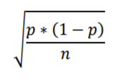
The variable p is the proportion rather than percentage: .5 rather than 50% (and 0 rather than 0%; .01 rather than 1%; .1 rather than 10%; and 1 rather than 100%).
The p * (1 – p) term in the numerator is called the proportion variance.
The variance p * (1 – p) reflects this dynamic:
- 0.0 * (1 – 0) = 0.00
- .01 * (1 – .01) = .01
- .1 *(1 – .1) = .09
- .3 *(1 – .3) = .21
- .5 *(1 – .5) = .25
- .7 *(1 – .7) = .21
- .9 *(1 – .9) = .09
- .99 *(1 – .99) = .01
- 1.0 *(1 – 1) = 0.00
So, as p moves from .5 towards 0 or 1, variance decreases, and since variance is in the numerator, Standard Error decreases. Decreases in Standard Error correspond to narrowing of the sampling distribution. This reflects lower uncertainty. Lower variance, lower uncertainty. Variance is itself a statistic and is very important in statistical analysis. We’ll be seeing it in formulas from now on. Now let’s consider sample size, which is represented in the denominator of the formula by n.
Larger sample sizes have narrower sampling distributions. Since n is in the denominator of the Standard Error formula, as n increases Standard Error decreases. Again, decreases in Standard Error correspond to narrowing of the sampling distribution. Again, this reflects lower uncertainty. Larger sample size, lower uncertainty.
Now we can use the Standard Error scale to determine 95% intervals. First, an important fact: The boundary lines of the 95% interval on the Standard Error scale are always -2 and +2 (they’re actually -1.95996… and +1.95996…, but I’m rounding to -2 and +2 for the present purposes). Let’s clarify all this by looking at several example calculations and illustrations.
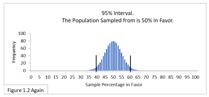
Let’s start with random sampling of 100 from a population that is 50% in favor of the new public health policy (Figure 1.2, below).
Plugging in the numbers gives
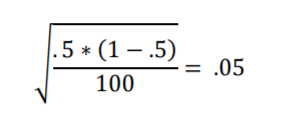
Standard Error is .05 and two Standard Errors is .1 in proportions and 10% in percentages. Since we want to center the interval on the percentage p of 50%, we’ll add and subtract 10% from 50%. This yields a calculated 95% interval of 50% + 10% (50% minus 10% to 50% plus 10%) or 40%-to-60%. That’s also what Figure 1.2 shows!
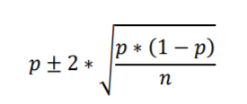
Putting everything we just computed into a formula for calculating 95% intervals we get
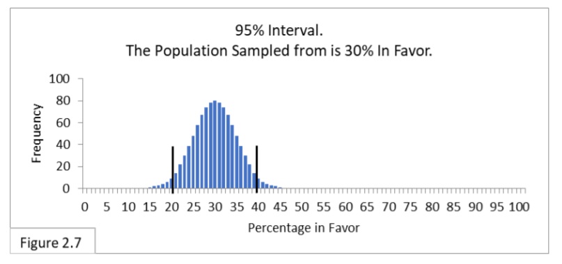
Next let’s consider the 95% interval of random sampling of 100 from a population that is 30% in favor of the new public health policy (Figure 2.7, reproduced below).

Standard Error is .045 and two Standard Errors is .09 in proportions and 9% in percentages. We want to center the interval on 30%, so we’ll add and subtract 9% from 30%. This yields a 95% interval of 30% ± 9% (30% minus 9% to 30% plus 9%) or 21%-to-39%. That’s also what Figure 2.7 shows!
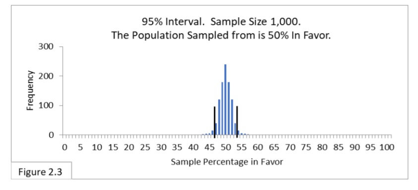
Last let’s consider the 95% interval of random sampling of 1000 from a population that is 50% in favor of the new public health policy (Figure 2.3, below).

Standard Error is .015 and two Standard Errors is .03 in proportions and 3% in percentages. We want to center the interval on 50%, so we’ll add and subtract 3% from 50%. This yields a 95% interval of 50% + 3% or 47%-to-53%. That’s also what Figure 2.3 shows!
The formula works! The reason the formula works is because the sampling distributions are “bell shaped”. More than that, they approximate the very special bell shape called the Normal distribution.
Let’s go one step further and standardize an entire sampling distribution to get what’s called the Standard Normal distribution. The Standard Normal Distribution is a normal distribution that uses Standard Error as its unit (rather than percentages or proportions). To illustrate, let’s standardize Figure 1.1 (below).
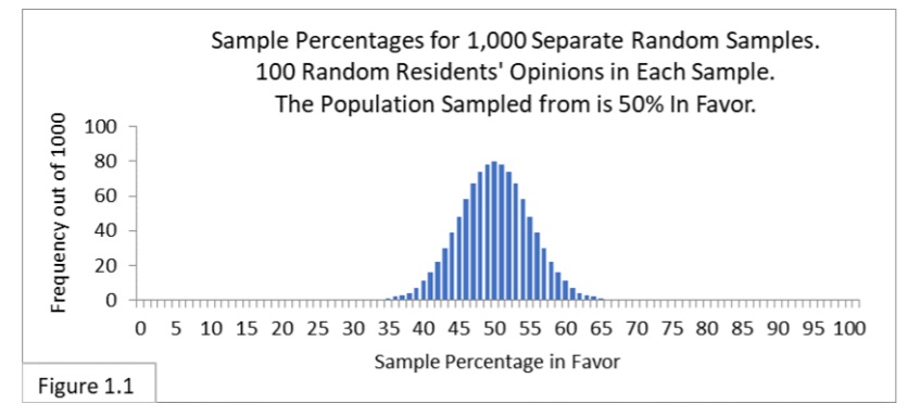
Figure 3.1 is a standardized version of Figure 1.1.
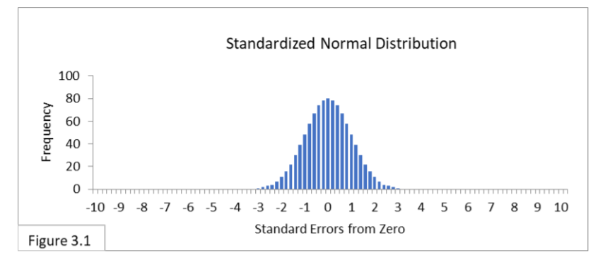
Notice that Standard Error is the unit used on the horizontal axis of Figure 3.1. This is done by rescaling the horizontal axis unit of Figure 1.1 to the Standard Error unit of Figure 3.1 using the below formula.
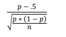
This formula gives us how many Standard Errors a proportion, p, is from .5. First, we convert the percentages to proportions. Next, we recenter the axis: whereas Figure 1.1 is centered on the proportion value .5 (50%), Figure 3.1 is centered on zero Standard Errors; the numerator p-.5 centers the horizonal axis of Figure 3.1 onto zero. Finally, these differences are divided by the Standard Error to rescale the horizontal axis. Voila, Figure 1.1 has been standardized to the Standard Error scale of Figure 3.1.
Figure 3.2 shows its 95% interval below Figure 1.2.

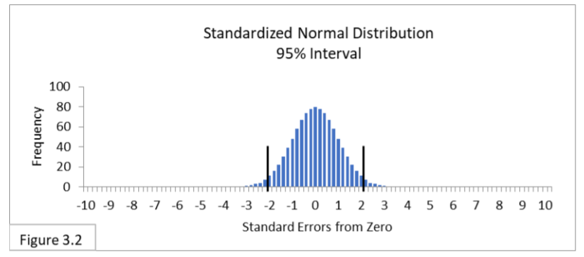
The boundary lines of the 95% interval on the Standard Error scale are -2 and 2 (rounded). Plugging .4 (40%) and .6 (60%) from Figure 1.2 into the above formula gives us -2 and 2 Standard Errors as the 95% boundary lines in the Standard Error unit. As emphasized above: The boundary lines of the 95% interval on the Standard Error scale are always -2 and +2 (rounded). If we standardized Figures 2.3 and 2.7,
we’ll again find the 95% interval boundary lines to be -2 and 2. (You can use the formula and do the arithmetic if you want to confirm this.)
We can convert our units (e.g., percent-in-favor, percent-heads) into the Standard Error unit and vice versa by multiplying and dividing by Standard Error. That comes in very handy. All of the sampling distributions we’ve looked at so far can be standardized in this way. In practice, we don’t convert entire sampling distributions to the standardized distribution; we use Standard Error in formulas as multipliers and divisors to calculate individual values, like we do to calculate the boundary lines for 95% intervals and to convert proportions to the Standard Error scale.
Check out our YouTube channel. You’ll find videos on the most popular topics. We’re adding more helpful tips every week. Comments are always welcome.
References
Kenney, J. F. and Keeping, E. S. Mathematics of Statistics, Pt. 1, 3rd ed. Princeton, NJ: Van Nostrand, 1962.
J.E. Kotteman. Statistical Analysis Illustrated – Foundations . Published via Copyleft. You are free to copy and distribute this content.
Zwillinger, D. (Ed.). CRC Standard Mathematical Tables and Formulae. Boca Raton, FL: CRC Press, 1995.
