Type I and Type II Error (Decision Error): Definition, Examples

> Statistics Definitions > Type I and Type II Error

Contents:

1. What is Type I Error?
2. What is Type II Error?
3. Examples of Type I and Type II Error

 

Type I & Type II Error: What is Type I Error?

A Type I error (or Type 1), is the incorrect rejection of a true null hypothesis. The alpha symbol, α, is usually used to denote a Type I error.

The null hypothesis, H₀ is a commonly accepted hypothesis; it is the opposite of the alternate hypothesis. Researchers come up with an alternate hypothesis, one that they think explains a phenomenon, and then work to reject the null hypothesis. If that sounds a little convoluted, an example might help. Back in the day (way back!) scientists thought that the Earth was at the center of the Universe. That meant everything else—the sun, the planets, the Oort cloud—revolved around the Earth.

 

This Geocentric model, where the Earth is at the center of the universe, has since been proven false. So the current, accepted hypothesis (the null) is:

• H₀: The Earth IS NOT at the center of the Universe.

And the alternate hypothesis (the challenge to the null hypothesis) would be:

• H₁: The Earth IS at the center of the Universe.

Type I Error: Conducting a Test

In our sample test (Is the Earth at the center of the Universe?), the null hypothesis is: H₀: The Earth is not at the center of the Universe Let’s say you’re an amateur astronomer and you’re convinced they’ve all got it wrong. You want to prove that the Earth IS at the center of the Universe. You set out to prove the alternate hypothesis and sit and watch the night sky for a few days, noticing that hey—it looks like all that stuff in the sky is revolving around the Earth! You therefore reject the null hypothesis and proudly announce that the alternate hypothesis is true; The Earth is, in fact, at the center of the Universe. That’s a very simplified explanation of a Type I Error. Of course, it’s a little more complicated than that in real life (or in this case, in statistics). But basically, when you’re conducting any kind of test, you want to minimize the chance that you could make a Type I error. In the case of the amateur astronomer, you could probably have avoided a Type I error by reading some scientific journals.

Type I & Type II Error: What is Type II Error?

A Type II error (sometimes called a Type 2 error) is the failure to reject a false null hypothesis. The probability of a type II error is denoted by the beta symbol β.

Let’s say you’re an urban legend researcher and you want to research if people believe in legends such as:

• Newton was hit by an apple (he wasn’t).
• Walt Disney drew Mickey mouse (he didn’t—Ub Werks did).
• Marie Antoinette said “Let them eat cake” (she didn’t).

The accepted fact is, most people probably believe in urban legends (or we wouldn’t need Snopes.com)*. So, your null hypothesis is:

• H₀: Most people do believe in urban legends.

But let’s say that null hypothesis is completely wrong. It might have been true ten years ago, but with the advent of the Smartphone—we have Snopes.com and Google.com at our fingertips. Still, your job as a researcher is to try and disprove the null hypothesis. So you come up with an alternate hypothesis:

• H₁: Most people DO NOT believe in urban legends.

You conduct your research by polling local residents at a retirement community and to your surprise you find out that most people do believe in urban legends. The problem is, you didn’t account for the fact that your sampling method introduced some bias: retired folks are less likely to have access to tools like Smartphones than the general population. So you incorrectly fail to reject the false null hypothesis that most people do believe in urban legends (in other words, most people do not, and you failed to prove that). You’ve committed an egregious Type II error, the penalty for which is banishment from the scientific community. *I used this simple statement as an example of Type I and Type II errors. I haven’t actually researched this statement, so as well as committing numerous errors myself, I’m probably also guilty of sloppy science.

Type I and Type II Error: Examples

We’ll start off using a sample size of 100 and .4 to .6 boundary lines to make a 95% confidence interval for testing coins. Any coin whose proportion of heads lies outside the interval we’ll declare unfair. Only 5% of the time will a fair coin mislead us and lie outside the interval, leading us to erroneously declare it unfair. This is Type I Error. What about unfair coins that mislead us and lie inside the interval? That will lead us to erroneously declare them fair. This is Type II Error. Let’s explore these two types of potential errors with some examples.

Imagine that I present you with a basket full of coins. The basket has an unknown number of fair coins and an unknown number of unfair coins. Your task is to test two arbitrary coins by flipping each one 100 times. You’re going to use the 95% interval to make your judgment: If the number of heads is within the .4-to-.6 interval then you’ll judge the coin to be fair, and if the number of heads is outside the .4-to-.6 interval then you’ll judge the coin to be unfair. Figure 4.1 highlights the four things that can happen with fair/unfair coins that are within/outside the 95% interval for the hypothesis that the coin is fair. 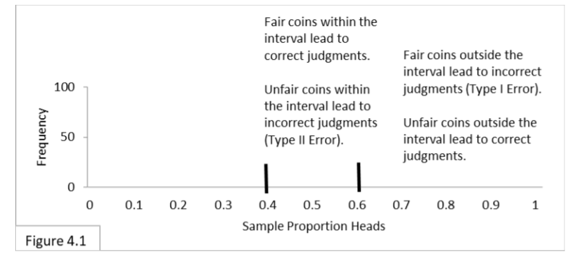Table 4.1 presents the information in a tabular format. (Some readers prefer the Figure and others prefer the Table, so I’m including both.) Let’s say you select a coin, flip it 100 times, and get a result of 55 heads. That’s inside the interval, so you judge the coin to be fair. If in fact the coin is fair, then the result is veridical(true) and leads you to make a correct judgment. If in fact the coin is unfair, then the result is misleading and leads you to make a Type II Error. Now let’s say you select another coin, flip it 100 times, and get a result of 65 heads. That’s outside the interval, so you judge the coin to be unfair. If in fact the coin is unfair, then the result is veridical (true) and leads you to make a correct judgment. If in fact the coin is fair, then the result is misleading and leads you to make a Type I Error. At first, many people think (hope) that using a 95% confidence interval means that there is a 95% chance they’re correct and a 5% chance they’re incorrect. But, unfortunately, that’s not what it means. Its meaning is much more limited. Our sampling distribution and its confidence interval portrays a very specific situation. In this case, it portrays the situation of flipping only fair coins. It does not portray flipping unfair coins. When we are in fact flipping fair coins, we do in fact expect that 95% of the outcomes will be within the .4-to-.6 boundary lines and 5% will be outside. But when we are in fact flipping unfair coins, this sampling distribution doesn’t tell us what to expect. What if all the coins in the basket are fair? Then you expect to be correct 95% of the time and to fall victim to Type I Error 5% of the time. Type II Error is irrelevant because it only applies to unfair coins. What if all the coins in the basket are unfair? Then Type I Error is irrelevant because it only applies to fair coins. And, we have no idea, at this point, how many times we should expect to be correct or how many times we should expect to fall victim to Type II Error. Our 95% interval has nothing definitive to say about unfair coins. If we knew, for example,

1. That ½ of the coins in the basket are fair and ½ are unfair, and
2. that the unfair coins are all identical and favor heads ¾ versus tails ¼,

then we could do some calculations to determine how likely it is that your judgments are correct. But we don’t know those things. We can make use of estimates of those things. In Frequentist statistics, we can, if we wish, estimate values for #2 in order to then estimate the likelihood of Type II Error. We’ll explore that next. But we do not make nor use estimates for #1. (Estimates for #1 are used to determine what’s called the false discovery rate.

Exploring Type II Error

Figure 4.2 shows the expected results of testing an unfair coin that comes up heads 30% (.3) of the time and tails 70% (.7) of the time.
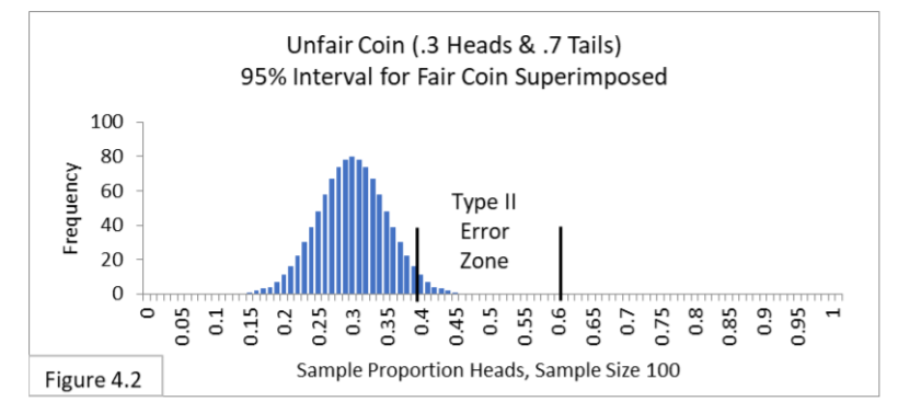
The person testing the coin has no knowledge of this. This person is testing whether the coin is fair and so is using a 95% interval for a fair coin that comes up heads 50% (.5) of the time and tails 50% (.5) of the time. Notice that the great majority of trials for the unfair coin will be outside the 95% interval for a fair coin and will lead to the correct judgment that the coin is unfair. However, about 2% of the time the unfair coin will be within the interval and be incorrectly judged to be fair. That is Type II Error. 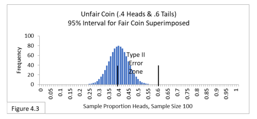Using your imagination, you can envision that if the unfair coin is closer to fair—say it comes up heads 40% (.4) of the time—then the bell shape will be farther to the right, so more of it will be between the boundary lines of .4-to-.6, and so there will be more frequent Type II Errors. Figure 4.3 illustrates what you might have imagined. The closer the unfair coin is to being fair, then the more Type II Errors we can expect. In Figure 4.3 about 50% of the trials are Type II Errors! What if we increase our sample size? The sampling distribution and the 95% interval get narrower when we increase sample size. Using your imagination, narrow the bell shape and the 95% interval of Figure 4.2. That should lead to fewer Type II Errors, shouldn’t it? Yes. Figure 4.4 illustrates what you might have imagined. With a larger sample size of 1000 (rather than 100) Type II Error seems extremely unlikely. 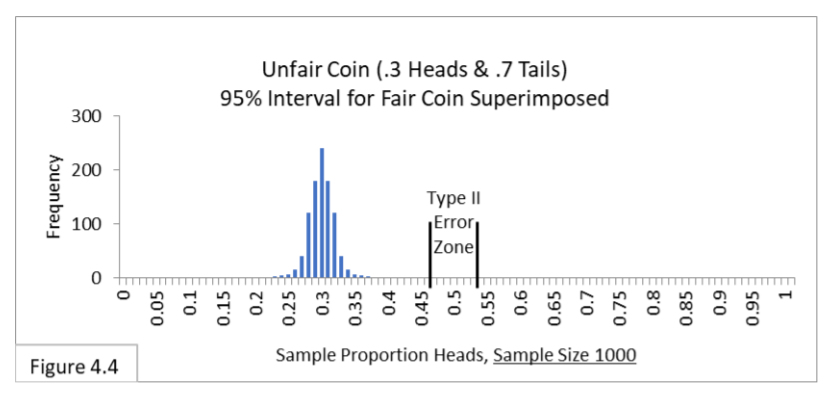In summary, the closer something is to what we’re testing for, and the smaller the sample size, the more likely we are to suffer Type II Error. There is another avenue to suffering higher Type II Error rates: making our Type I Error criterion stricter.

99% Intervals and Their Effects on Type I and Type II Error

While 95% intervals are the most commonly used (except in sciences such as particle physics), some researchers argue for stricter lines to be drawn: in particular, they argue for use of 99% intervals to better avoid Type I Errors (particle physicists use even stricter lines). Figure 4.5 shows the 99% interval for a fair coin and a sample size of 100.
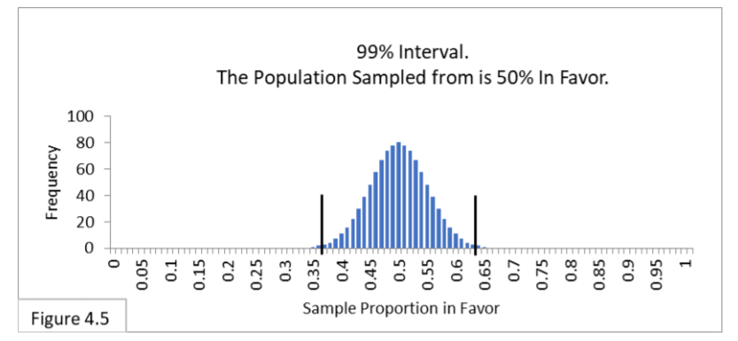
With a 99% interval, 99% of the expected sample proportion values with fair coins are contained within the interval. Since it contains more of the expected outcomes than the 95% interval, it is wider. In this case the boundary lines are .37-to-.63 (wider than the .40-to-.60 we have with our 95% interval). Now only 1% of the expected values are outside the boundary lines, ½% on each side. With a wider interval, our sample statistic value needs to be more extreme in order to fall outside the interval. In that way, it is a stricter criterion with respect to Type I Error. We can use the stricter criterion to lessen the chances of Type I Error. But what happens with Type II Error? As you might expect, since you can’t get something for nothing, Type II Error will become more likely. First, look at Figure 4.6 shown below.
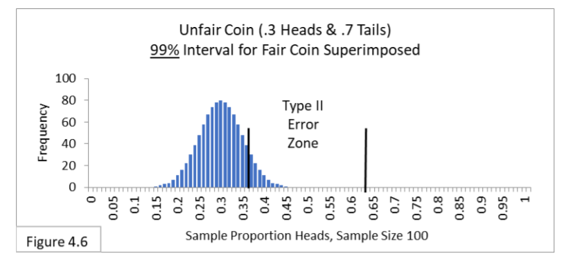
As you can see when comparing Figure 4.6 with Figure 4.2 (reproduced below), more outcomes of the same unfair coin are now within the 99% interval than were within the 95% interval. This is not a surprise since the 99% interval is wider. Whereas about 10% of the unfair coins result in Type II Error with the 99% interval, only about 2% of the unfair coins result in Type II Error with the 95% interval. In short: When we make our Type I Error criterion stricter, we increase the likelihood of Type II Error. In practice, we determine the acceptable likelihood of Type I Error by the confidence interval we choose to use—95% and 99% intervals are the most common in the social sciences, whereas 99.9999% is used in particle physics.

As we’ve just seen, the likelihood of Type II Error is determined by a number of factors, some within our control and some not. In summary, the likelihood of Type II Errors increases:

1. the closer something is to what we’re testing for (.4 is closer to .5 than .3 is, and so .4 coins make Type II Errors more likely than .3 coins). We don’t control this.
2. when we use smaller sample sizes (a sample size of 100 makes Type II Errors more likely than a sample size of 1000). We do control this, although larger samples cost more to gather.
3. when we use stricter Type I Error criteria (a 99% interval is stricter for Type I Error and makes Type II Error more likely than a 95% interval—but keep in mind that Type I Error becomes less likely; it’s a trade-off). We do control this, but in practice the strictness of our Type I Error criteria is usually set by convention (social sciences use 95% and sometimes 99%; physical sciences use 95% through 99.9999% depending on the specific field).

Decreasing the likelihood of Type II Error increases the statistical power of our analysis. In practice, increasing the sample size is a common way to reduce the likelihood of Type II Error. Moreover, there are formulas and software tools (including online calculators) available that help researchers estimate what their sample size should be in order to achieve their desired levels of Type I and Type II Error. With these tools you enter your estimated value for the population proportion, your expected sample proportion value, and your desired Type I and II Error rates. Keep in mind that, since you don’t actually know what the population proportion is nor what your sample proportion will be, the sample size recommendations of these tools are “educated-guess” estimates.

In practice, Type I Error is feared more than Type II Error. In the social sciences the Type I Error limit is most often set at 5% via a 95% confidence interval. With surveys, for example, we want to limit how often we infer that a majority of the population is in favor of a new policy when in fact a majority is not in favor. What about Type II Error? That occurs if we infer that a majority of the population is not in favor of the new policy when in fact a majority is in favor. There is no well established convention, but the most common guidance is to try and limit Type II Error to 20% (by having large enough sample sizes). These guidelines of 5% and 20% imply that we prefer to error on the conservative side, maintaining the status quo. Using our surveying context, this means that statistical survey evidence is more likely to erroneously undermine new policies than to erroneously provide support for them. While 95% and 99% intervals are common, much stricter Type I Error criteria are used in particle physics: 99.9999% (approximately). Using this interval with coin flipping, we would insist that a coin come up heads at least 75 times in 100 flips before declaring it unfair. Biologists conducting what are called genome-wide association studies use a similarly strict interval. Since these researchers test hundreds of thousands or even millions of separate genome locations, Type I Errors would be expected to occur far too frequently if they used a 95% or 99% interval. After all, 5% of 1,000,000 is 50,000 and 1% of 1,000,000 is 10,000.

References

Everitt, B. S.; Skrondal, A. (2010), The Cambridge Dictionary of Statistics, Cambridge University Press.
Kanji, G. K. 100 Statistical Tests. Thousand Oaks, CA: SAGE Publications, p. 110, 1999.
Lindstrom, D. (2010). Schaum’s Easy Outline of Statistics, Second Edition (Schaum’s Easy Outlines) 2nd Edition. McGraw-Hill Education
Vogt, W.P. (2005). Dictionary of Statistics & Methodology: A Nontechnical Guide for the Social Sciences. SAGE.
J.E. Kotteman. Statistical Analysis Illustrated – Foundations . Content published via Copyleft. You are free to copy and distribute the content of this article.