Calculus Problem solving is a wide topic covering hundreds of possibilities from finding lengths and areas to calculating rates of change and continuity of functions.
Calculus Problem Solving: Contents
Click on a topic to go to that article:
- Analytic Geometry:
- Business:
- Derivatives:
- Functions:
- Average Value of a Function
- Basic Operations on Functions
- Check the Continuity of a Function
- Decompose a Composite Function
- Express x as a function of y
- Function Intervals: Decreasing/Increasing
- How to Find Intercepts
- Parametric to Rectangular Forms
- Quadratic Formula
- Relation vs Function
- Vertical Shift of a Function
- See also: Functions (main page).
- Integrals:
- Limits:
- Determining Limits From a Graph
- Finding Area by the Limit Definition
- See also: Limit of Functions (main page).
- Optimization
- Physics:
- Pre-Calc:
- Curve Sketching
- Eliminate exponents
- Symbols and Equations (How to Read Them)
- See also: Precalculus (main page).
- Sequence and Series:
- Volume:
- Word Problems Index
- TI 89 Calculus: Step by Step
The Tautochrone Problem / Brachistrone Problem
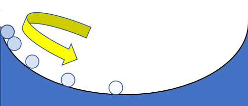
The tautochrone problem addresses finding a curve down which a mass placed anywhere on the curve will reach the bottom in the same amount time, assuming uniform gravity. The solution, discovered in May 1697 by at least five different mathematicians, is an (inverted) cycloid [1]. A similar problem is the brachistochrone problem, which asks the question: What is the curve of fastest descent? The solution is also a cycloid.
History of the Tautochrone Problem
The tautochrone problem goes back to the time of Galileo (1564-1642), who discovered that large, high-speed pendulum swings or small, low-speed swings take about the same length of time. He later realized he could use the principle to construct a clock, but he lacked the mechanical skills needed to actually build one. Later on, Christiaan Huygens (1629-1695) constructed the first working model of the cycloidal pendulum. Several of his pendulum clocks to determine longitude at sea were built and tested in 1662. In his book, Horologium Oscillatorium, Huygens proved that the cycloid is tautochronous [3], which means “occupies the same time”.
During his study of pendulums, Huygens discovered that a ball rolling back and forth on an inverted cycloid completes a full “swing” in exactly the same amount of time. He solved the tautochrone problem without calculus, using Euclidean geometry [4]. In addition to the cycloid, there are an infinite number of tautochrone curves which are solutions to the problem [5]. One way to solve the problem is with Laplace Transforms [6].
What is the Integral Transform?
The integral transform is a way to solve challenging problems by transforming coordinates into another space, via integration, where the problem is easier to solve. The solution is then transformed back into the original coordinates with an inverse transform.
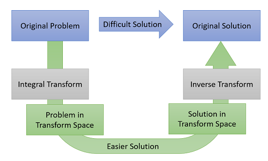
Integral transforms are applied to Initial Boundary Value Problems (IBVP) as follows [1]:
- Apply a transform to one independent variable of the partial differential equation. This eliminates any partial derivatives associated with that variable.
- Solve the transformed PDE (if this isn’t possible, the equation can be transformed again).
- Invert the transforms to convert the solution to the solution of the original IBVP.
Types of Integral Transform
There are an infinite number of transforms. The most commonly used transforms in calculus are the Laplace transform and the Fourier transform. Fourier transforms are widely used in engineering and physics, while the Laplace transform is an efficient way of solving some ordinary and partial differential equations. However, there is really only one difference between the two methods: Laplace transforms can be defined for unstable systems with the Fourier transform cannot [2]. They are named after the mathematicians who originally worked on them: Laplace and Fourier.
Other types of commonly used transformations include:
- Fourier-cosine transform,
- Fourier-sine transform,
- Hankel transform,
- Mellin transform.
Which one you use is usually determined by the boundary condition. For example, the ideal transformation a problem defined on a semi-infinite domain (0, ∞) in space with a Dirichlet boundary condition is the Fourier sine transform.
Formal Definition of Integral Transform
More formally, the integral transform with integral kernel K is a mapping that takes function f(t) to a function f(x) with the rule [3]:
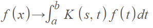
Where a and b are real numbers (including infinity and negative infinity).
Integral Transform: References
[1] Lambers, J. (2013). Integral Transforms (Sine and Cosine Transforms). Retrieved May 10, 2021 from: https://www.math.usm.edu/lambers/mat417/lecture8.pdf
[2] M. Shehu & Weidong, Z. New Integral Transform: Shehu Transform a Generalization of Sumudu and Laplace Transform for Solving Differential Equations. Retrieved May 10, 2021 from: http://arxiv-export-lb.library.cornell.edu/pdf/1904.11370
[3] Green, L. (2020). The Laplace Transform. Retrieved May 9, 2021 from: https://math.libretexts.org/Bookshelves/Analysis/Supplemental_Modules_(Analysis)/Ordinary_Differential_Equations/6%3A_Power_Series_and_Laplace_Transforms/6.6%3A_The_Laplace_Transform
Calculus Problem Solving Example: Path of a Baseball
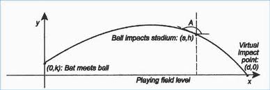
The path of a baseball hit by a player is called a parabola. Its graph can be represented in calculus using a pair of parametric functions with time as the dimension. These functions depend on several variables, including:
- The height from the ground at which the baseball was hit,
- Its angle of elevation with the horizontal,
- The initial velocity of the baseball when hit.
Wind speed is another factor that will affect the path of the baseball, but this factor forms complex equations and is not dealt with in these simplified parametric equations.
Path of a baseball: Steps
Step 1: Define the variables used in both the parametric equations.
- Represent the height in feet by ‘h’,
- The angle in degrees by ‘a’,
- The initial velocity in feet per second by ‘v’
- The time in seconds by ‘t’.
Step 2: Write an equation for the horizontal motion of the baseball as a function of time:
- x(t) = v * Cos(a) * t.
Step 3: Write an equation to describe the vertical motion of the baseball as a function of time:
- y (t) = h + v * Sin(a) * t – 16 * t2.
In this formula, t2 is the square of the variable ‘t’, which is simply t * t, or t2.
The pair of x(t) and y(t) equations are the required parametric equations that describe the path of the baseball in calculus.
Tips:
- If the initial velocity is known with the unit of miles per hour (mph), it can be converted to the required unit of feet per second (fps) unit. 5280 feet make a mile, 60 minutes make an hour and 60 seconds make a minute. Accordingly, the mph value has to be multiplied by 1.467 to get the fps value.
- The value of the trigonometric functions Cos(a) and Sin(a) can be found by using a look-up table or simply by using a calculator. If the ball was hit along the ground, the angle ‘a’ is zero.
References
[1] Malo, R. (2016). The Tautochrone Problem. Retrieved April 11, 2021 from: https://math.montana.edu/malo/172f16/Tautochrone.pdf
[2] Larson, R. & Edwards, B. (2009). Calculus, 9th Edition. Brooks Cole.
[3] MacTutor. Christiaan Huygens. Retrieved April 11, 2021 from: https://mathshistory.st-andrews.ac.uk/Biographies/Huygens/#:~:text=Huygens%20was%20elected%20to%20the,with%20a%20spring%20regulated%20clock.
[4] Swift, J. Cycloid. Retrieved April 11, 2021 from: https://oak.ucc.nau.edu/jws8/dpgraph/cycloid.html
[5] Pedro, T. et al. Is the tautochrone curve unique? Retrieved April 11, 2021 from: https://ui.adsabs.harvard.edu/abs/2016AmJPh..84..917T/abstract
[6] Gulas, M. (2018). The Pope’s Rhinoceros and Quantum Mechanics. Retrieved April 11, 2021 from: https://scholarworks.bgsu.edu/cgi/viewcontent.cgi?article=1469&context=honorsprojects
Wiggle Graphs
A wiggle graph (or sign graph) is a segmented number line that describes where a function is increasing or decreasing. Derivatives give information about where a function is headed as well, so the wiggle graph is also a way to visualize the signs of a function’s derivative. It’s called a wiggle graph because it tells you where the function is “wiggling” towards.
How to Draw a Wiggle Graph
Example question: Draw a wiggle graph for the function:
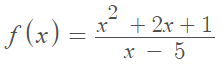
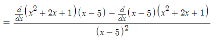
Step 1: Find the first derivative. For this particular function, use the quotient rule.
 Applying the quotient rule.
 Simplifying
 Applying the quotient rule.
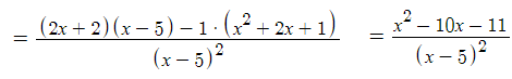 Simplifying
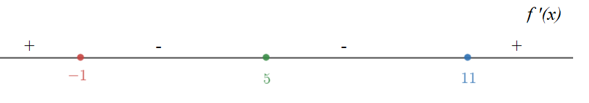
Step 2: Find the critical values for the function. Critical values are where the first derivative is equal to zero, or is undefined.
The derivative we calculated in Step 1,
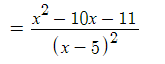
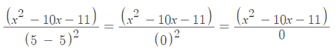
will be undefined if the denominator is equal to zero (because of division by zero). This happens when x = 5:
We can factor the numerator to find out when the derivative will equal zero:
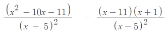
When x = 11 or x = -1, the numerator will be zero, making the fraction equal zero.
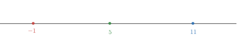
Therefore, we have three critical values: x = -1, x = 5, and x = 11
Step 3: Draw a number line and label it with your critical values. Do not write any other numbers on the line. This doesn’t have to be drawn to scale:
Step 4: Choose a number for each interval on the graph you drew in Step 3. We have four intervals in this example, labeled A, B, C, and D in this image:
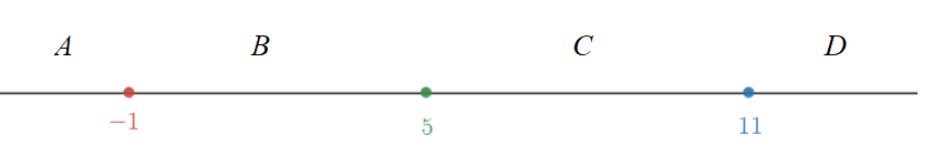
It doesn’t matter what numbers you choose, as long as you pick one from each interval. To make calculations relatively easy, I’ll pick -3, 1, 10 and 12.
Step 5: Plug the values you chose in Step 4 into the derivative from Step 1:
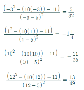
Step 6: Label the wiggle graph with the signs of the first derivative. Add the label “f′(x)” to make it clear this wiggle graph is for the first derivative:
The completed wiggle graph tells us that the function is increasing on the first interval, decreasing on the second and third intervals, and increasing on the fourth.