Taylor’s Theorem; Lagrange Form of Remainder

Calculus Problem Solving >

Taylor’s Theorem is a procedure for estimating the remainder of a Taylor polynomial, which approximates a function value. In other words, it gives bounds for the error in the approximation. The remainder given by the theorem is called the Lagrange form of the remainder [1].

Formula for Taylor’s Theorem

The formula is:


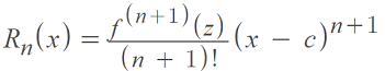
Where:

• R_n(x) = The remainder / error,
• f⁽ⁿ⁺¹⁾ = The nth plus one derivative of f (evaluated at z),
• c = the center of the Taylor polynomial.

The equation can be a bit challenging to evaluate. In many cases, you’re going to want to find the absolute value of both sides of this equation, because of the challenges involved in evaliating the higher derivative: you normally have to take an educated guess here and there for the value of “z”: Sometimes, graphing the function may help with that step, as in the following example.

Taylor Theorem Example

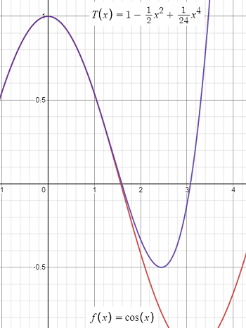
Example Question: What is the expression for the remainder for the following Maclaurin polynomial approximation of f(x) = cos(x) for cos(0.2)?

Step 1: Identify the degree of the polynomial. This is a 4th degree. We can tell that by the highest degree in the equation (the last term is to the 4th power). It’s also identified as T₄ on the left side of the equation.

Step 2: Add 1 to Step 1.
4 + 1 = 5.

Step 3: Fill in the formula with what you know so far:

• c is 0, because all Maclaurin polynomials are centered at zero.
• (n + 1) is the number from Step 2 (for this example, that’s 5).
• x = 0.2 (this is given in the question: we’re finding the approximation for cos(0.2)).

Step 4: Evaluate the numerator f⁵ (z). In English, that is telling us to “evaluate the fifth derivative of the function at point z”. Our function is cos(x):
f⁵ cos(x) = -sin(x).
The problem is we can’t directly evaluate it for z (we don’t know what “z” is!). But we do know (from looking at the graph above, in this example), that the cosine function has function values ranging from -1 to 1.

This is where taking the absolute value of both sides comes in. Rather than trying to work with -1 to 1, we can just work with the absolute value of the max function value, which in this case, is 1. We can then rewrite our formula as an inequality:


Evaluating this on a calculator, we get:
|R₄cos(0.2)| = 0.0000026666.

This is a tiny error, which is what we would expect from the graph.

Note: If we reevaluate for cos(2), you would get 0.26666666666, which is a much larger error. This is an upper bound for the error though; In reality the error here is much smaller (around 0.2).

Why is Taylor’s Theorem Useful?

In practice, the theorem is quite useful. The idea behind it is that a function’s true value is the Taylor approximation T_n(x) plus an error (remainder)— a measure of how far off the mark the approximation is. If we can find bounds (i.e. a min or max) for the size of f^{(n + 1)}(x) on the interval (a, b), then we can use the theorem to get concrete error estimates for any Taylor approximation.[2]

References

Graph: Desmos.com.
[1] Larson, R. & Edwards, B. (2017). Calculus. 11th Edition. Cengage Learning.
[2] Generalizing the Mean Value Theorem – Taylor’s theorem. Retrieved April 26, 2021 from: https://ocw.mit.edu/courses/mathematics/18-01sc-single-variable-calculus-fall-2010/unit-2-applications-of-differentiation/part-c-mean-value-theorem-antiderivatives-and-differential-equations/session-34-introduction-to-the-mean-value-theorem/MIT18_01SCF10_ex34sol.pdf