What are Boundary Conditions?
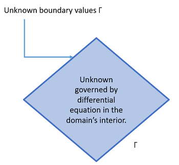
Differential equations have many solutions and it’s usually impossible to find them all. To narrow down the set of answers from a family of functions to a particular solution, conditions are set. These conditions can be initial conditions (which define a starting point at the extreme of an interval) or boundary conditions (which define bounds that constrain the whole solution). Different types of boundary conditions can be imposed on the boundary of a domain.
One way to think of the difference between the two is that initial conditions deal with time, while boundary conditions deal with space. Boundaries can describe all manner of shapes: e.g. triangles, circles, polygons.
Types of Boundary Conditions
The five types of boundary conditions are:
- Dirichlet (also called Type I),
- Neumann (also called Type II, Flux, or Natural),
- Robin (also called Type III),
- Mixed,
- Cauchy.
Dirichlet and Neumann are the most common.
- Dirichlet: Specifies the function’s value on the boundary. For example, you could specify Dirichlet boundary conditions for the interval domain [a, b], giving the unknown at the endpoints a and b. For two dimensions, the boundary conditions stretch along an entire curve; for three dimensions, they must cover a surface. This type of problem is called a Dirichlet Boundary Value Problem..
- Neumann: Similar to the Dirichlet, except the boundary condition specifies the derivative of the unknown function. For example, we could specify u′(a) = α which imposes a Neumann boundary condition at the right endpoint of the interval domain [a, b].
- Robin: A weighted combination of the function’s value and its derivative. For example, for unknown u(x) on the interval domain [a, b] we could specify the Robin condition u(a) −2u′(a) = 0.
- Mixed: Similar to the Robin, except that parts of the boundary are specified by different conditions. For example, on the interval [a, b], the unknown u′(x) at x = a could be specified by a Neumann condition and the unkownn u(x) at x = b could be specified by a Dirichlet condition. [1]
- Cauchy: Similar to the Robin, except that while the Robin condition implies only one constraint, the Cauchy condition implies two.
Homogeneous boundary conditions are set to zero; Otherwise they are called inhomogeneous.
Examples
When solving a differential equation, the values for the conditions depend on the problem you’re trying to solve.
As an example, let’s say you wanted to find the equation for a straight line on a curve-length function between two points (a, A) and (b, B). The function could be set up as with the points as boundary conditions [2]:
![]()
Where y′ = a constant.
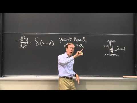
Watch the following video from MIT courseware that overviews boundary conditions and shows two more examples:
References
[1] Introduction to Boundary Value Problems. Retrieved March 20, 2021 from: https://people.sc.fsu.edu/~jpeterson/bvp_notes.pdf
[2] Open University. Introduction to the calculus of variations.