Degrees of Freedom: Definition, Examples

Hypothesis testing > Degrees of freedom

What are Degrees of Freedom?

When it comes to statistical data, the term degrees of freedom (df) is a measure of how much freedom you have when selecting values for your data sample. More specifically, it is the maximum number of values that can be independently varied in a given sample.

Let’s say you were finding the mean weight loss for a low-carb diet. You could use four people, giving three degrees of freedom (4 – 1 = 3), or you could use 100 people with df = (100 – 1) = 99. As a formula,  where “n” is the number of items in your sample:

Degrees of Freedom = n – 1

Watch the video for an overview:

Can’t see the video? Click here to watch it on YouTube.

Contents:

1. Calculations / Formulas
2. Why do we subtract 1 from the number of items?
3. Degrees of freedom: Two Samples
4. Degrees of Freedom in ANOVA
5. Why Do Critical Values Decrease While DF Increase?
6. History of Degrees of Freedom

 

Calculations / Formulas

There are many ways of calculating degrees of freedom, depending on the tests. In basic statistics, you’ll use the basic formula (subtracting 1), but as you progress with statistics you’ll come across different formulas.

• Single sample test (e.g., one sample t-test): df = N – 1, where N is the number of items in your data sample. For example, if your sample contains four items, your degrees of freedom would be 3 (4 – 1 = 3). 
• For comparing multiple groups (e.g., ANOVA): df = k – 1, where k is the number of groups being compared. For example, if you are comparing the mean weight loss for 3 diet plans using between groups, df = 3 – 1 = 2.
• When you estimate k parameters (e.g., regression analysis): N – k. In some tests, degrees of freedom for the “residual” or “error” is N – k. For example, if you want to fit k parameters to N data points in linear regression with k coefficients, the residual degrees of freedom is N – k. 

Not all degrees of freedom are whole numbers. Some special cases, like the T-distribution, allow decimals instead of whole numbers. In other situations, like when working with an entire population instead of a sample, degrees of freedom might not be needed at all.

Why do we subtract 1 from the number of items?

The answer to this question lies in how many values that are free to vary. What does “free to vary” mean? Consider an example using the mean (average):

• Choose a set of numbers with a mean (average) of 10. A. Some possible sets of numbers include: 9, 10, 11 or 8, 10, 12 or 5, 10, 15.
• Once you’ve selected the first two numbers in the set, the third one becomes fixed. In other words, you cannot choose the third item in the set freely. The only numbers that can vary freely are the first two. You can select 9 + 10 or 5 + 15, but once you’ve made that decision, you must choose a specific number that will result in the desired mean. Therefore, the degrees of freedom for a set of three numbers is two.

For example, when finding a confidence interval for a sample, the degrees of freedom are n – 1, where ‘n’ represents the number of items, classes, or categories. Once we have chosen one category/class/item, we reduce our “free to vary” items by 1.

We only subtract 1 for single sample analysis. For two samples, subtract 2, using this formula:

Degrees of Freedom (Two Samples): (N₁ + N₂) – 2.

Note that if you do Welch’s t‐test (unequal variance), the df formula is more complicated and generally not an integer.

Back to Top

Degrees of Freedom: Two Samples

If you have two samples and want to find a parameter, like the mean, you have two “n”s to consider (sample 1 and sample 2). Degrees of freedom in that case is:

Degrees of Freedom (Two Samples): (N₁ + N₂) – 2.

In a two sample t-test, use the formula df = N – 2 because there are two parameters to estimate.

Back to Top

Degrees of Freedom in ANOVA

Degrees of freedom become slightly more complex in ANOVA tests. Unlike a simple parameter (such as a mean), ANOVA tests involve comparing known means within data sets. For instance, in a one-way ANOVA, you compare two means in two cells. The grand mean (the average of the averages) would be:

Mean 1 + Mean 2 = grand mean.

If you chose Mean 1 and knew the grand mean, you wouldn’t have a choice regarding Mean 2, so your degrees of freedom for a two-group ANOVA is 1.

Two Group ANOVA df1 = n – 1

Potential confusion: In most cases, n is the total sample size. However, some sources or course notes use “n” to mean the number of groups. For example, if you have 2 groups then 2 – 1 = 1. Double check to see which variation your instructor / textbook is using.

For a three-group ANOVA, you can vary two means, so the degrees of freedom are 2.

In reality, it’s a bit more complicated because there are two degrees of freedom in ANOVA: df1 and df2. The explanation above is for df1. In ANOVA, df2 is the total number of observations in all cells minus the degrees of freedom lost because the cell means are set.

Two Group ANOVA df2 = n – k

In this formula, “k” represents the number of cell means or groups/conditions. For example, let’s say you had 200 observations and four cell means. Degrees of freedom in this case would be: Df2 = 200 – 4 = 196.

Back to Top

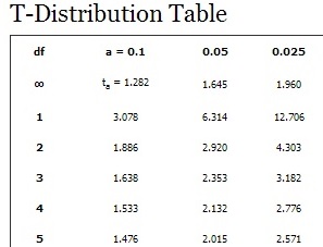
Why Do Critical Values Decrease While DF Increase?

Let’s take a look at the t-score formula in a hypothesis test:
When n increases, the t-score goes up. This is because of the square root in the denominator: as it gets larger, the fraction s/√n gets smaller and the t-score (the result of another fraction) gets bigger. As the degrees of freedom are defined above as n-1, you would think that the t-critical value should get bigger too, but they don’t: they get smaller. This seems counter-intuitive.

However, think about what a t-test is actually for. You’re using the t-test because you don’t know the standard deviation of your population and therefore you don’t know the shape of your graph. It could have short, fat tails. It could have long skinny tails. You just have no idea.

The degrees of freedom affect the shape of the graph in the t-distribution; as the df get larger, the area in the tails of the distribution get smaller. As df approaches infinity, the t-distribution will look like a normal distribution. When this happens, you can be certain of your standard deviation (which is 1 on a normal distribution).

Let’s say you took repeated sample weights from four people, drawn from a population with an unknown standard deviation. You measure their weights, calculate the mean difference between the sample pairs and repeat the process over and over. The tiny sample size of 4 will result a t-distribution with fat tails. The fat tails tell you that you’re more likely to have extreme values in your sample. You test your hypothesis at an alpha level of 5%, which cuts off the last 5% of your distribution.

The graph below shows the t-distribution with a 5% cut off. This gives a critical value of 2.6. (Note: I’m using a hypothetical t-distribution here as an example–the CV is not exact). 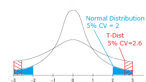Now look at the normal distribution. We have less chance of extreme values with the normal distribution. Our 5% alpha level cuts off at a CV of 2. Back to the original question “Why Do Critical Values Decrease While DF Increases?” Here’s the short answer:

Degrees of freedom are related to sample size (n-1). If the df increases, it also stands that the sample size is increasing; the graph of the t-distribution will have skinnier tails, pushing the critical value towards the mean.

Back to Top

History of Degrees of Freedom

English statistician Ronald Fisher popularized the idea of degrees of freedom.  He is credited with explicitly defining the degrees-of-freedom concept, beginning with his 1915 paper on the distribution of the correlation coefficient [1]. His discovery of degrees of freedom was due in part by an error made by Karl Pearson, claimed that no correction in degrees of freedom are needed when parameters are estimated under the null hypothesis [2].

Fisher did not mince words when it came to Pearson’s error: In a volume of his collected works, Fisher wrote about Pearson, “If peevish intolerance of free opinion in others is a sign of senility, it is one which he had developed at an early age” [3].

Although Fisher is credited with the development of degrees of freedom in 1915, Carl Friedrich Gauss introduced the basic concept as early as 1821 [4]. However, its modern definition is thanks to English statistician William Sealy Gosset in his 1908 Biometrika article “The Probable Error of a Mean“, published under the pen name “Student.” While Gosset [Student]did not use the term ‘degrees of freedom,’ he did explain the concept while developing Student’s t-distribution. Gosset and Fisher were in correspondence together and Fisher proved a geometrical formulation that Gosset had been working on [5].

In sum, key events in the history of degrees of freedom include:

• 1820s: Adrien-Marie Legendre further develops the least squares method.
• 1870s: William Sealy Gosset creates the t-distribution.
• 1900s: Ronald Aylmer Fisher develops the chi-square distribution.
• 1920s: Jerzy Neyman and Egon Pearson establish hypothesis testing.
• 1930s: Harold Hotelling formulates confidence intervals.
• 1940s: John Tukey develops robust statistics.
• 1950s: William Kruskal and William Wallis create nonparametric statistics.
• 1960s: John W. Tukey introduces exploratory data analysis.
• 1970s: John Hartigan develops the bootstrap.

Another way to look at Degrees of Freedom

If you still can’t wrap your head around the concept, don’t beat yourself up. Even the great Karl Pearson couldn’t hone in on its meaning without making an error! Many authors throughout the years have pointed out the esoteric nature of the term, including Walker [6], who said in 1940 that “For the person who is unfamiliar with N-dimensional geometry or who knows the contributions to modern sampling theory only from secondhand sources such as textbooks, this concept often seems almost mystical, with no practical meaning.”

According to Joseph Lee Rogers of Vanderbilt university [1], a simpler way to look at degrees of freedom is that it defines an accounting process that counts the flow of data from the statistical bank — into which we deposit data points — into the model. When you run a statistical analysis involving parameters (e.g., a t test or regression analysis), you withdraw money from the bank to pay for estimating the parameters in your model. Degrees of freedom is a count of the statistical money you have withdrawn from the bank and the statistical money still left in the bank.

References

1. Rodgers JL. Degrees of Freedom at the Start of the Second 100 Years: A Pedagogical Treatise. Advances in Methods and Practices in Psychological Science. 2019;2(4):396-405. doi:10.1177/2515245919882050
2. Stigler, S. Karl Pearson’s Theoretical Errors and the Advances They Inspired. Statistical Science, 2008, Vol. 23 No. 2, 261-271.
3. Agresti, A. Historical Highlights in the Development of Categorical Data Analysis.
4. Walker H. M. (1940). Degrees of freedom. Journal of Educational Psychology, 31, 253–269.
5. Sir Ronald Aylmer Fisher.
6. Fisher R. A. (1915). Frequency distribution of the values of the correlation coefficient in samples from an indefinitely large population. Biometrika, 10, 507–521.