Contents:
1. What is Stationarity?
A time series has stationarity if a shift in time doesn’t cause a change in the shape of the distribution. Basic properties of the distribution like the mean , variance and covariance are constant over time.

Types of Stationary
Models can show different types of stationarity:
- Strict stationarity means that the joint distribution of any moments of any degree (e.g. expected values, variances, third order and higher moments) within the process is never dependent on time. This definition is in practice too strict to be used for any real-life model.
- First-order stationarity series have means that never changes with time. Any other statistics (like variance) can change.
- Second-order stationarity (also called weak stationarity) time series have a constant mean, variance and an autocovariance that doesn’t change with time. Other statistics in the system are free to change over time. This constrained version of strict stationarity is very common.
- Trend-stationary models fluctuate around a deterministic trend (the series mean). These deterministic trends can be linear or quadratic, but the amplitude (height of one oscillation) of the fluctuations neither increases nor decreases across the series.
- Difference-stationary models are models that need one or more differencings to become stationary (see Transforming Models below).
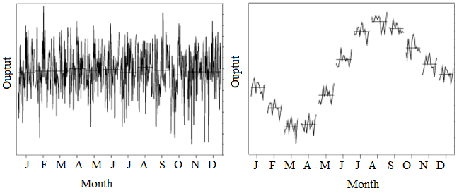
It can be difficult to tell if a model is stationary or not. Unlike the obvious example showing seasonality above, you usually can’t tell by looking at a graph. If you aren’t sure about the stationarity of a model, a hypothesis test can help. You have several options for testing, including:
- Unit root tests (e.g. Augmented Dickey-Fuller (ADF) test or Zivot-Andrews test),
- A KPSS test (run as a complement to the unit root tests).
- A run sequence plot,
- The Priestley-Subba Rao (PSR) Test or Wavelet-Based Test, which are less common tests based on spectrum analysis.
Why is Stationarity Important?
Most forecasting methods assume that a distribution has stationarity. For example, autocovariance and autocorrelations rely on the assumption of stationarity. An absence of stationarity can cause unexpected or bizarre behaviors, like t-ratios not following a t-distribution or high r-squared values assigned to variables that aren’t correlated at all.
Transforming Models
Most real-life data sets just aren’t stationary. To quote Thomson (1994):
“Experience with real-world data, however, soon convinces one that both stationarity and Gaussianity are fairy tales invented for the amusement of undergraduates.”
To put it another way, if you’ve got a real-life data set (and not a theoretical one from a class), you’re going to need to make it stationary in order to get any useful predictions from it. A model can sometimes be stationarized through mathematical transformation (usually performed by software) which makes the model relatively easy to predict; It will have the same statistical properties at a later date. The mathematical transformations are then reversed so that the new model predicts the behavior of the original time series model. Transformations might include:
- Difference the data: differenced data has one less point than the original data. For example, given a series Zt you can create a new series Y
i = Zi – Zi – 1. - Fit a curve to the data, then model the residuals from that curve.
- Take the logarithm or square root (usually works for data with non-constant variance).
Some models can’t be transformed in this way — like models with seasonality. These can sometimes be broken down into smaller pieces (a process called stratification) and individually transformed. Another way to deal with seasonality is to subtract the mean value of the periodic function from the data.
2. Differencing
Differencing is where your data has one less data point than the original data set; You’re subtracting (or moving) a point—a “difference”. For example, given a series Zt you can create a new series Yi = Zi – Zi – 1. As well as its general use in transformations, differencing is widely used in time series analysis.
“A series with no deterministic component which has a stationary, invertible ARMA representation after differencing d times is said to be integrated of order d…(Engle and Granger 1987, p. 252.)”
In calculus, differencing is used for numerical differentiation. The general idea is similar (e.g. with backwards differencing you are subtracting a point), but the applications are different. While differencing in calculus still involves “moving” a point, the movement is so that you can estimate a derivative (i.e. the slope).
References:
Engle, R. F. and Granger, C. W. J. (1991) Long-run Economic Relationships: Readings in Cointegration, Oxford University Press.
Priestley, M. & Subba Rao, T. (1969) A Test for Non-Stationarity of Time-Series. Journal of the Royal Statistical Society. Series B (Methodological), Vol. 31, No. 1, pp. 140-149.
Von Sachs, R. & Neumann, M. (2000). A Wavelet-Based Test for Stationarity. Journal of Time Series Analysis. Vol. 21, No. 5. September, pp. 597-613.
Thomson, D.J. 1994. Jackknifing multiple-window spectra. In: Proceedings of the IEEE International Conference on Acoustics, Speech and Signal Processing, VI, 73-76.