Contents:
- What is Monte Carlo Simulation?
- Quantified Probability and Real-Life Uses
- Accuracy
- Simple Example
- The Splitting Method
- Software & MATLAB Example
- Histogramming
1. What is Monte Carlo Simulation?
Monte Carlo simulation (also called the Monte Carlo Method or Monte Carlo sampling) is a way to account for risk in decision making and quantitative analysis. The method finds all possible outcomes of your decisions and assesses the impact of risk. It was invented during the Manhattan Project by John von Neumann and Stanislaw Ulam and named for Ulem’s uncle who enjoyed playing games of chance in Monte Carlo, Monaco.
The technique uses intensive statistical sampling methods that are so complex they are usually only performed with the aid of a computer. The procedure is complex for several reasons:
- The input model is simulated hundreds or thousands of times (or sometimes hundreds of thousands of times), where each end simulation is equally likely. The result is a probability distribution of possible outcomes. This could be one, or many different distributions including the normal distribution, chi-squared distribution, uniform distribution, or one of dozens more different probability distributions.
- Monte Carlo transforms numbers from a random number generator, and sequences of these transformed numbers will repeat after a certain number of samples. While error in calculating statistics (like the mean) will become acceptable, the errors will not vanish completely or become insignificant. This violates the Central Limit Theorem and The Law of Large Numbers (Fishman, 1996), two theorems that are the underpinnings of the “usual” statistics most people are comfortable with. If absolute accuracy is your goal, this method isn’t for you, but if you’re looking for numbers that are “in the ballpark” with at best a 5-10% error, then this may be a good choice.
The Monte Carlo method tells you:
- All of the possible events that could or will happen,
- The probability of each possible outcome.
As far as the Manhattan project went, one of the possible events that could have happened was that the atomic bomb caused a chain reaction that blew up the world. The probability was calculated as being so improbable that it was impossible (that said, the simulation did account for the possibility!).
2. Quantified Probability and Real-Life Uses
The Monte Carlo simulation returns a quantified probability, which means that it gives you scenarios with numbers you can use. Let’s say you’re company wants to know if local bird life will be adversely affected by the construction of a new factory close to wetlands. A quantified probability would be “If we build the factory, there is a 30% chance the nesting bird population will be adversely affected.” This is more useful that a more general, qualified statement like “If we build the factory, the nesting bird population will be affected”.
Monte Carlo simulations are used in many areas of industry and science, including:
- Analyzing radiative heat transfer problems (Wang et.al),
- Estimating the transmission of particles through matter (Biersack & Haggmark),
- Calculating the probability of cost overruns in large projects (McCabe),
- Foreseeing where prices of securities are likely to move (Boyle et. al),
- Analyzing how a network or electric grid will perform in different scenarios. For example, Sortomme et. al ran simulations for how electric vehicle charging will affect the electric drig in the future.
- Assessing risk for credit or insurance (Gordy).
- Simulating proteins in biology (Earl et. al)
3. Accuracy
While a Monte Carlo simulation provides some good accuracy, it is unlikely to hit the “exact” mark for several reasons:
- Vast amounts of data are usually involved.
- There are usually several unknowns in the system.
- As it is probabilistic (i.e. randomness plays a role in predicting future events), there will always be a margin of error related to the results.
In fact, it can be quite easy to run a “bad” Monte Carlo simulation (Brandimarte, 2014). This can happen for a variety of reasons, including:
- Use of an incorrect model or an unrealistic probability distribution,
- The underlying risk factors aren’t complete (i.e. you haven’t specified them well enough),
- The choice of Monte Carlo (which uses a stochastic model) isn’t suited to your data,
- The random number generator chosen for the method isn’t good enough,
- Computer bugs, which you may not be aware of if your area of expertise is statistics (as opposed to programming).
4. Simple Example of How Monte Carlo Works
Example 1. Odds of Blackjack

- Ten of clubs / Ace of clubs
- Jack of clubs / Ace of clubs
- Queen of clubs / Ace of clubs
- Jack of clubs / Ace of clubs…
If you wrote down all of the possible combinations of cards (including all those combinations of two cards that don’t add up to 21, you would find the probability of getting a Blackjack is about 1:21. In other words, the probability of getting a blackjack is one in twenty-one hands. With small numbers, like a deck of cards, figuring out your sample space (i.e. all of the possible outcomes) is fairly simple and doesn’t take a lot of time. But if you have a larger number of inputs — say, thousands of cards, then figuring out a sample space using a probabilistic method like this one becomes unwieldy. Enter the Monte Carlo method.
Another way of figuring out the probability of getting a Blackjack is to choose two cards a set number of times (say, one hundred times) and record the outcomes. The more times you take a sample of two cards, the closer you’ll get to the “real” figure of 1:21. For example, if you choose two cards a thousand times you’re probably going to get very close to 1:21; If you choose two cards a dozen times, you probably won’t get close at all — you might get a run of “luck” or you might get no “21s” at all. This is essentially how Monte Carlo simulations work. Instead of writing out the sample space (which is what we did in the first part of this example), Monte Carlo samples and locates the most likely outcome, creating a stochastic model. The fact that Monte Carlo uses a very simple draw (in this example, two cards), and repeats it over and over again, is why the method is sometimes called The Method of Statistical Trials.
Back to Top
5. The Splitting Method
The splitting method is a Monte Carlo simulation for rare events or for sampling from high-dimensional data. The program takes a complex scenario and “splits” it up into easy-to-calculate parts. On a basic level, the program makes the event more likely to occur so that a probability distribution can be found.
6. Software & MATLAB EXAMPLE
A wide variety of software has been developed to run Monte Carlo simulations. These include:
- General-purpose programming languages (e.g. C++, Java, or Visual Basic),
- Spreadsheet add-ins (e.g. Excel),
- Statistical software packages (e.g. R, MATLAB, R, and SPSS).
- Graphical editors (e.g. Simulink and Arena20).
MATLAB Example 2: Collecting Letters
When I first backpacked across the States in the 1980s, McDonald’s was running a promotion where you had to collect little paper Monopoly pieces stuck to the sides of Super Size fries and drinks. Despite knowing the odds were not in my favor, my younger self couldn’t resist purchasing Super Size Fish Filet meals in order to try and win. I think the most I won was a large fry, but it serves to illustrate the power of these marketing techniques.
Usually, the game is really about who is lucky enough to get the rare pieces. In 2016, the rare pieces included Mayfair for £100,000 cash (UK) or Boardwalk for $1,000,000 (US). For this example code, it’s assumed there is an equal chance of getting every playing piece.
> nLetters = 9; %BIGMACFRY
> nTrials = 10000;
> for i=1:nTrials
> success = 0;
> nTries(i) = 0;
> for j=1:nLetters
> BIGMACFRY(j)=0; %reset letter not achieved
> end
> while success == 0
> nTries(i) = nTries(i)+1; %inc. count
> buy = 1+floor(nLetters*rand); %letter obtained
> BIGMACFRY(buy) = 1;
> if sum(BIGMACFRY)==nLetters
> success = 1;
> end
> end
> end
> hist(nTries)
(MATLAB code modified from Shonkwiler & Mendivil, “Explorations in Monte Carlo Methods”)
7. Histogramming
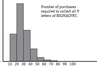
Histogramming is a popular way to show results from Monte Carlo simulations. The following histogram shows the results from the above Monopoly piece simulation.

The histogram reveals a couple of surprising results:
- It could take 100 purchases to get all 9 pieces.
- The number of purchases peaks after the minimum (which, if you get a lucky streak, is 9); the model then decreases exponentially.
References:
Biersack & Haggmark. A Monte Carlo computer program for the transport of energetic ions in amorphous targets. Nuclear Instruments and Methods. Volume 174, Issues 1–2, 1 August 1980, Pages 257-269. Retrieved August 26, 2017 from: Science Direct.
Boyle et. al. Monte Carlo methods for security pricing. Journal of Economic Dynamics and Control
Volume 21, Issues 8–9, 29 June 1997, Pages 1267-1321. Retrieved August 26, 2017 from: http://www.sciencedirect.com/science/article/pii/S0165188997000286
Brandimarte, P. (2014). Handbook in Monte Carlo Simulation: Applications in Financial Engineering, Risk Management, and Economics. Wiley.
Earl et. al. Monte Carlo Simulation. Molecular Modeling of Proteins pp 25-36. Retrieved August 26, 217 from: https://link.springer.com/protocol/10.1007/978-1-59745-177-2_2
Fishman, G. (1996). Monte Carlo. Springer Science & Business Media.
Gordy. A comparative anatomy of credit risk models. Journal of Banking & Finance
Volume 24, Issues 1–2, January 2000, Pages 119-149. Retrieved August 2017 from: http://www.sciencedirect.com/science/article/pii/S0378426699000540
McCabe, B. Construction engineering and project management III: monte carlo simulation for schedule risks. WSC ’03 Proceedings of the 35th conference on Winter simulation: driving innovation. Pages 1561-1565. Retrieved August 26, 2017 from: ACM Digital Library.
Shonkwiler & Mendivil. Explorations in Monte Carlo Methods. 2009. Springer.
Sortomme et. al. Coordinated Charging of Plug-In Hybrid Electric Vehicles to Minimize Distribution System Losses. IEEE Transactions on Smart Grid. March 2011. Volume: 2 Issue: 1
Wang et. al. Monte Carlo simulation of radiative heat transfer and turbulence interactions in methane/air jet flames. Journal of Quantitative Spectroscopy and Radiative Transfer.
Volume 109, Issue 2, January 2008, Pages 269-279. Retrieved August 26 2017 from: http://www.sciencedirect.com/science/article/pii/S0022407307002464