< Descriptive Statistics < Skewness
Contents:
The articles explain specific measures of skew in more detail:
What is Skewness?
Skewness is a measure of the asymmetry of a probability distribution. In other words, it tells you how “off center” a non-symmetrical distribution is.
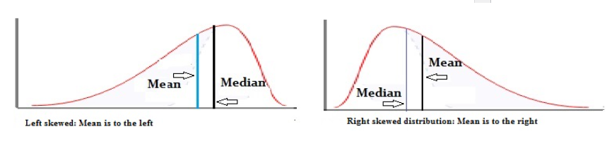
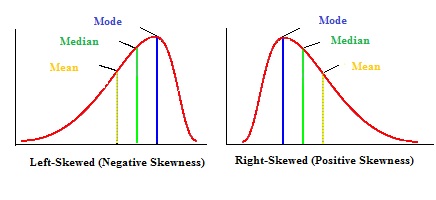
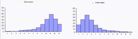
- A left-skewed distribution has a long left tail and is sometimes called a negatively skewed distribution because it’s long tail is on the negative direction on a number line.
- A right-skewed distribution has a long right tail and is sometimes called a negatively skewed distribution because it’s long tail is on the positive direction on a number line.
Skew is used in conjunction with kurtosis to better predict the probability of events occurring in the tails of a probability distribution. It also tells you where the bulk of outliers are, although it doesn’t tell you how many there are in a distribution. If the distribution is right-skewed, most of the outliers are on the right side of the distribution, while if it is left-skewed, most of the outliers are on the left.
Equations
The following table shows the equations for calculating the skew for various distributions you’re likely to come across in elementary statistics. Note that the normal, Student’s T, uniform and Laplace distributions are not shown on the table as they are not skewed.
| Distribution. | Equation. |
|---|---|
| Bernoulli distribution. | |
| Beta distribution. | |
| Binomial distribution. | |
| Chi square distribution. | |
| F distribution. | |
| Negative binomial. | |
| Poisson Distribution. |
Calculation
The skewness formula given in many textbooks is Pearson’s First Coefficient of Skewness:
Skew = (Mean – Median) / Standard Deviation.
Another common way is with Pearson’s Second Coefficient of Skewness:
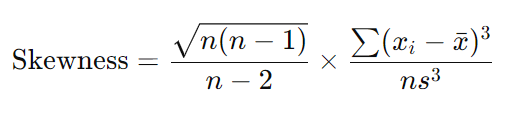
Skew = 3 (Mean – Mode) / Standard Deviation.
In Pearson’s Second Coefficient, the mode (not the median) is used. This coefficient is specifically designed to work in cases where the mode is known or can be estimated.
If outliers or a long tail are of concern, the Pearson mode formula might be more appropriate because the mean can be highly affected by outliers.
If you are comparing the skewness of two or more distributions that have different sample sizes, then you should adjust for sample size because because the second coefficient can be biased for small samples. T
The adjusted Fisher-Pearson skewness coefficient adjusts for sample size:
How to interpret skewness values
- A value of 0 means that the distribution is symmetric.
- A value greater than 0 means that the distribution is positively skewed.
- A value less than 0 means that the distribution is negatively skewed.
Acceptable values fall between − 3 and + 3 [1].
The typical acceptable range often cited is between -2 and +2 for moderate skewness, though some sources, especially for financial or economic data, might accept a range between -3 and +3 as reasonable, depending on the context.
That said, a “good” value for skew depends on the data. For example, a professor might want to see a high positive skew value (0.1. or larger) for their class’s final exam scores (meaning that more students would score As), while a negative skew smaller than -0.3 would be much more preferable for distribution of incomes (which means that there would be fewer “big earners” and more of an equitable distribution of wealth).
Let’s look at some real-life examples:
- Income distribution is positively skewed. A small number of individuals earn very high incomes, while the majority earn significantly less.
- Height distribution is generally symmetrical with zero skew. Most people are around the average height and fewer at the extremes (very tall or very short).
- Test scores vary in skewness. Test scores are often negatively skewed if the test is easy, meaning most students score high. For more challenging tests, they may be positively skewed, with a few high scorers and most scoring lower.
- Waiting times often have positive skew. Waiting times often have a long right tail, with most people waiting a short time and a few waiting much longer. Negative skew would suggest the opposite, which is less common.
Example: What does a skew of 1.67 mean?
It means that the distribution is positively skewed, with more data in a long tail extending to the right. A value of 1.67 is quite high (the maximum skew is 3), and it is often indicative of a heavily skewed distribution.
What is Momental Skewness?
Momental skewness is one of four ways you can calculate the skew of a distribution. It’s called “Momental” because the first moment in statistics is the mean. The formula for calculating momental skewness (γ) is: α(m) = 1/2 γ1 = μ3 / 2 σ3 Where μ is the mean and σ is the standard deviation and γ is the Fisher Skewness.
Why use Momental Skewness?
Which technique you use depends on what you know about your data. For example, if you know the mean, mode (or median) and standard deviation you can use Pearson’s. Momental skewness could be an option if you only know the mean and standard deviation for your set of data.
What do the Results Mean?
A symmetrical distribution has a skew of zero. A positive result means that your data is positively skewed. A negative results means that your data is negatively skewed. Momental skewness will give you a result that is half of typical skewness. Back to Top
Skewness in Excel
When you calculate skewness in Excel, Excel will return a positive or a negative number. A normal distribution, which has perfectly symmetrical tails, has a skewness of zero.
You have two different options for calculating skewness in Excel 2013: the SKEW function or Data Analysis (How to load the Data Analysis Toolpak). If you’re taking a statistics class, it would be worth your while to install the Toolpak as it gives you access to many stats functions that aren’t in the base installation of Excel.
SKEW Function
- Type your data into columns.
- Click an empty cell on the worksheet.
- Type “=SKEW(xx:yy)” where xx:yy is the cell location of your data (for example, C1:C25).
Data Analysis
- Click the “Data” tab and then click “Data Analysis.”
- Click “Descriptive Statistics” and then click “OK.”
- Click the Input Range box and then type the location for your data. For example, if you typed your data into cells A1 to A10, type “A1:A10” into that box
- Click the radio button for Rows or Columns, depending on how your data is laid out.
- Click the “Labels in first row” box if your data has column headers.
- Click the “Descriptive Statistics” check box.
- Select a location for your output. For example, click the “New Worksheet” radio button.
- Click “OK.”
Skewness in Minitab
Skewness in Minitab:
- Click “Stat”, then click “Basic Statistics,” then click “Descriptive Statistics.”
- Click the variables you want to find the median for and then click “Select” to move the variable names to the right window.
- Click “Statistics.”
- Check the “Skewness” box and then click “OK” twice.
Excel, Minitab and most other modern software packages use the adjusted Fisher-Pearson standardized moment coefficient to find skew. The results of the calculation tell you:
- The direction of the skew (positive or negative).
- How the sample compares with a normal (symmetric) distribution. The further the skew result is from zero, the greater the skew
Check out our YouTube channel for more stats help and tips!
References
- Brown, T. A. (2006). Confirmatory factor analysis for applied research. Guilford Press.