Contents:
- Principal Component Analysis
- Canonical Correlation Analysis (CCA)
- Correspondence Analysis
- Redundancy Analysis
What is Principal Component Analysis?
Principal Component Analysis (PCA) is a tool that has two main purposes:
- To find variability in a data set.
- To reduce the dimensions of the data set.
Reducing dimensions means that redundancy in the data is eliminated; This can make patterns in the data set more clear. Therefore, Principal Component Analysis is a good tool to use if you suspect you have redundancy in your data set. Redundancy doesn’t mean that the variables are identical; it means that there is a strong correlation between them. For example, let’s say you are conducting a customer service survey with the following four questions where customers rate their satisfaction on a scale of 1 to 10:
- Shipping time was satisfactory.
- I received my item when I expected to receive it.
- The item was as described.
- The item fit the need that I purchased it for.
Questions 1 and 2 are concerning time, and questions 3 and 4 are concerning the actual item purchased. If you ran Principal Component Analysis on this simple example, the four separate variables could theoretically be reduced to two (time and cost). In real life, data sets could contain hundreds or thousands of variables, making redundancy impossible to identify. That’s where Principal Component Analysis comes in; it clears the “noise” to allow you to identify patterns in the data.
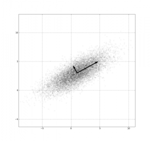
Principal Component Analysis reduces dimensions by projecting the whole data set onto a completely separate space. The original variables are transformed into a new set of artificial ones, which are the “Principal Components” of Principal Component Analysis. These components can be extremely useful as criterion variables or predictor variables in later data analysis.
Principal Component Regression (PCA)
Principal Component Regression is based on Principal Component Analysis. It is used when your data set exhibits multicollinearity. This means that although least squares estimates are biased, variances may be too far away from the actual value. PCA adds some bias to the regression model and reduces standard error. The first step in PCA is the same as in Principal Component Analysis: identify the principal components. Regression is then performed on those components.
PARAFAC
Parallel Factor Analysis (PARAFAC) is a generalization of Principal Component Analysis to higher-order arrays. It’s useful for exploratory data analysis on very particular sets of data, for example if you have three-way data (i.e. scores on n persons on m variable measured at p occasions1). Where PARAFAC differs from Principal Component Analysis is that PARAFACE produces unique components.
What is Correspondence Analysis?
Correspondence Analysis (CA) is a special case of PCA. PCA explores relationships between variables in tables with continuous measurement, while Correspondence analysis is used for contingency tables. Contingency tables are a way to represent data sets that fall into two or more categories.
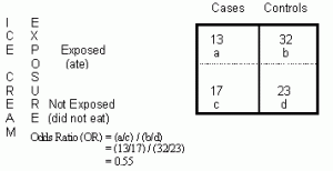
Correspondence Analysis can be used for everything from simple two-way tables to more complex, multi-way tables. CA is highly useful for more complex situations, as it simplifies the data and provides a detailed description of nearly every piece of information gleaned from the data. It’s primary function is to produce a graphical display containing “points” that represent rows and columns. The goal is to produce an overall view of the data in a low-dimensional space (i.e. a 2D graph) that is easy to interpret.
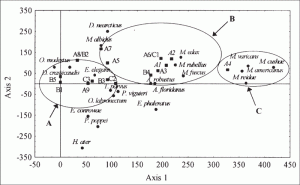
Mathematically, Correspondence Analysis is a way to break down the chi-square statistic into components due to the contingency table’s rows and columns. In more simple terms, it’s a way to assign order to categories.
Multiple Correspondence Analysis
Multiple Correspondence Analysis is an extension of CA for investigating the relationships between several categorical dependent variables. It should be used when you your observed data set is described by a number of nominal variables with several levels. Each level should have a binary code. For example, if you have a level for retired/not retired, retired could be “0” and not retired could be “1”. The inputs for MCA are via a Burt Table.
Alternative names for this technique include: dual scaling, optimal scaling, and quantification method. In technical terms, Multiple Correspondence Analysis is performed by using CA on an indicator matrix (or design matrix); Rows are cases and columns are categories of variables. The two main differences in the output are:
- Interpretation of inter-point differences must be modified.
- Percentages of explained variances has to be corrected.
What is Canonical Correlation Analysis (CCA)?
Canonical Correlation Analysis is one way to find associations between two data sets. Like the Correlation Coefficient, CCA measures the relationship between variables. Where Canonical Correlation Analysis differs is that it is specifically used to find the relationships between two sets of variables.
For example, an educational researcher may want to find the association between different measures of scholastic ability and success in school.
It’s appropriate to use CCA in the same situations as you might use multiple regression analysis, but when you have multiple intercorrelated outcome variables. CCA is not recommended for small data sets. Similar multivariate analysis methods include:
- Multivariate Multiple Regression, which is an alternative if you are not interested in dimensionality (canonical dimensions are identical to the factors in Factor Analysis).
- Separate Ordinary Least Squares Regressions, one for each variable in a set. However, this option would not produce multivariate results and also will not give you any information about dimensionality.
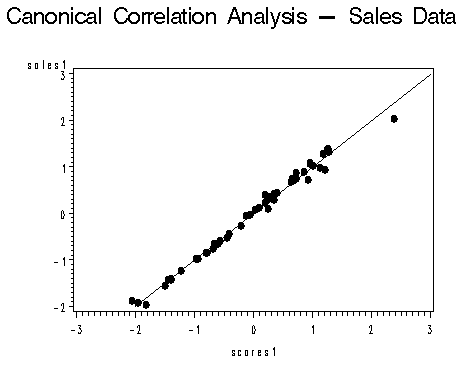
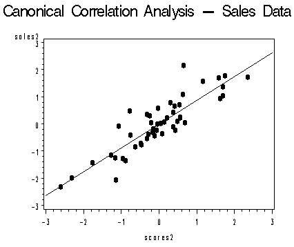
The purpose of Canonical Correlation Analysis is to explain the variability within and between sets through identification of several sets of canonical variates. Canonical variates are new variables formed by making a linear combination of two of more variables from the data sets. When running CCA, you choose weights that maximize the correlation between these sets of variates.
The following two images of canonical variates are taken from an SAS generated plot. They show two canonical variate pairs, graphed against a regression line to see how well the pairs fit (source: PSU.edu).
Real-Life Example
Canonical Correlation Analysis can be used in experiments to compare two sets of variables to see what they have in common. For example, you could compare two well known psychology personality tests, the Minnesota Multiphasic Personality Inventory (MMPI) and the Revised NEO Personality Inventory. When you compare the sets with CCA, you’ll be able to see how the MMPI’s factors relate to the NEOs factors. This results in you being able to see what the tests have in common and what variance is shared between the tests. For example, you might find that a fair amount of aggressiveness or introversion is shared between the tests.
What is Redundancy Analysis?
Redundancy Analysis is the constrained version of Principal Components Analysis. Constrained basically means reduction of dimensions. This reduction is what leads to more understandable results.
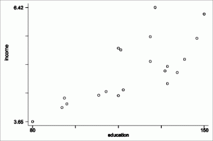
Redundancy Analysis is a way to summarize linear relationships in a set of dependent variables that are influenced by a set of independent variables. It is an extension of multiple linear regression. The method uses a blend of linear regression and Principal Components Analysis(PCA).
- Linear regression is first applied to represent Y as a function of X.
- PCA is then applied to a matrix of the results to provide a visual representation.
Redundancy Analysis is similar to Canonical Correlation Analysis. In both CCA and Redundancy Analysis, the correlation for components extracted from tables is maximized. However, they are maximized in slightly different ways:
- In Canonical Correlation Analysis, components are extracted from both tables so that correlations are maximized.
- In Redundancy Analysis, components of X are extracted from tables so that they are at a maximum correlation with Y. Then components of Y are extracted so that they are at a maximum correlation with X.
Assumptions for Redundancy Analysis
As Redundancy Analysis is an extension of linear regression, the same assumptions apply. For example, before performing Redundancy Analysis to a set of data you should check linear dependence. For example:
- Increasing X-values should result in increasing Y-values.
- If X-variables are doubled, then Y-values should also double.
In addition, the number of explanatory variables (independent variables) must be less than the number of objects in your data matrix. Your independent variables and dependent variables should also have the same physical units. If they don’t you should standardize them (i.e. find their z-scores) before running Redundancy Analysis. An exception is raw count data, which should not be standardized.
Related Articles
References
PSU.edu image retrieved Dec 14, 2020 from: https://onlinecourses.science.psu.edu/stat505/node/69
