Multiple Imputation for Missing Data: Definition, Overview

Statistics Definitions >

Multiple imputation (MI) is a way to deal with nonresponse bias — missing research data that happens when people fail to respond to a survey. The technique allows you to analyze incomplete data with regular data analysis tools like a t-test or ANOVA. Impute means to “fill in.” With singular imputation methods, the mean, median, or some other statistic is used to impute the missing values. However, using single values carries with it a level of uncertainty about which values to impute. Multiple imputation narrows uncertainty about missing values by calculating several different options (“imputations”). Several versions of the same data set are created, which are then combined to make the “best” values.

Advantages of Multiple Imputation

Used correctly, MI can:

• Reduce bias. “Bias” refers to errors that creep into your analysis.
• Improve validity. Validity simply means that a test or instrument is accurately measuring what it’s supposed to. For example, when you create a test or questionnaire for depression, you want the questions to actually measure depression and not something else (like anxiety).
• Increase precision. Precision is how close two or more measurements are to each other.
• Result in robust statistics, which are resistant to outliers (very high or very low data points).

Calculating Imputations

With the multiple imputations method, missing values are replaced by m > 1 possibilities, where m is usually < 10.

The general, very simplified, procedure (as outlined by Rubin, 1987) is a series of steps:

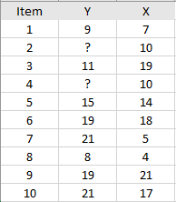
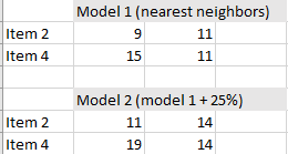
1. Fit your data to an appropriate model. Model fitting takes data from samples and attempts to find the best fit model, like a normal distribution or chi-square distribution. The model could also be some other parametric model gleaned from your data. For the above table, two simple models were created (giving two imputations): nearest neighbor, which took the values for the neighbor above and the neighbor below and nearest neighbor + 25%, which increased the nearest neighbor values to account for nonresponse bias.
2. Estimate a missing data point using the selected model. For example, the nearest neighbor model might generate a 9 for missing value Y2. 9 is the value found in one of the nearest neighbors (Y1).
3. Repeat steps 1 and 2 (you can use the same model, or different models) 2-5 times for each missing data point (this gives you multiple options for the missing data).





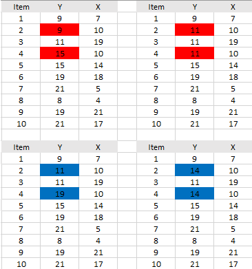
4. Perform your data analysis. For example, you might want to run a t-test, or an ANOVA. The test should be run across all missing data point sets. This example generated the four sets below, so your chosen tests would be run four times (once for each set).




5. Average the values of the parameter estimates, variances or standard errors obtained from each model to give a single point estimate for that model. In other words, you can combine the results from the two data sets generated from model 1, and you can also combine the results from the two data sets generated from model 2.

Although the simplified example above might seem intuitive, the calculations for approximating missing values are surprisingly complex. They involve:

• Bayesian analysis, which combines prior information about a parameter of interest with new evidence from a sample.
• Resampling from predicted distributions, where large numbers of smaller samples of the same size are repeatedly drawn, with replacement, from a single original sample.

Not only are multiple possibilities for the missing values calculated, but each suggested value can come from a different probability distribution. This analysis is practically impossible by hand without a good grasp of Bayesian methodology. Schafer (1999) warns that

“…a naïve or unprincipled imputation method may create more problems than it solves, distorting estimates, standard errors and hypothesis tests.”

To avoid these pitfalls, Rubin (1991) recommends that imputations should:

1. Apply a prior probability distribution to any unknown parameters using Bayesian analysis, simulating m independent draws from the conditional distribution of Y_missing given Y_observed by Bayes’ theorem,
2. Specify a parametric model for the complete data,
3. Specify (if possible) a model for the underlying mechanism causing the missing data.

Using Software

Most popular statistical software packages have options for multiple imputation, which require little understanding of the background Bayesian workings. For example, the IBM SPSS MI procedure is basically a point-and-click:

• Choose Analyze > Multiple Imputation.
• Select >2 variables for the model.
• Specify the number of imputations. The default value is 5.
• Specify the dataset or data file for your output.

Other popular software options include:

• R: Analytics Vidhya has a nice roundup of several R packages that deal with missing data, including multiple imputations.
• SAS: Use PROC MI or PROC MIANALYZE procedures.

Using software isn’t a perfect solution. Care should be taken to choose appropriate models for your data. For example, if your data isn’t normally distributed, you may need to transform your variables so that they approximate a normal distribution before running an imputation procedure. In other words, it isn’t as simple as inputting your data and clicking a multiple imputation option. Incorrect model choices, failure to include moderating variables, or excluding vital data points can all lead to even more bias than you would have had without running the procedure in the first place.

Other Options for Missing Data

No one “perfect” method exists for filling in missing data. As outlined above, multiple imputations can be difficult to understand and implement without some understanding of model selection and Bayesian theory. Some other options, which are simpler and may be more efficient than MI, include:

• Replace missing values with the mean or median for the set. Generally not recommended unless you have just a few missing values.
• Use linear regression to fill in the blanks. Linear regression creates a simple model (a line) where it’s easy to extrapolate or interpolate missing values. Only suited for data that is likely to be linear, like height, weight, or income levels.
• Replace missing values with the value before it. This may work if your values seem to have a trend (as opposed to values that are all over the place).
• Ignore cases with missing data, or weight the complete cases (i.e. give more importance to complete data and less importance to incomplete data). Ignoring cases with missing data may be an option if you’ve got a large enough sample size. For smaller samples, every data point may be critical.
• Fill in the blank areas with zeros. Mostly an option if you have a few, non-critical missing points.
• Use a k-nearest neighbor or EM algorithm to generate missing data points. Nearest neighbor matching logically matches one data point with another, most similar, data point. The EM algorithm works by choosing random values for the missing data points, and using those guesses to estimate a second set of data. The new values are used to create a better guess for the first set, and the process continues until the algorithm converges on a fixed point.

Further Reading:
For an in-depth look at MI, you really can’t beat D. B. Rubin’s original work Multiple imputation for nonresponse in surveys (New York: John Wiley, 1987). If you can’t find the book, you can read a pdf of Rubin’s MI method here.

References:
Little RJA & Rubin DB (2002) Statistical analysis with missing data (second edition). Wiley, NJ.
Rubin, D.B. (1977). Inference and missing data. Biometrika, 63, 581-592.
Rubin, D.B. (1978). Multiple Imputations in Sample Surveys — a phenomenological Bayesian approach to nonresponse. Proceedings of the survey research methods section of the American Statistical Association, 20-34. Also in imputation and editing of faulty or missing survey data, U.S. Dept. of Commerce, 1-23.
Rubin, D.B. (1986). Basic ideas of multiple imputation for nonresponse. Survey methodology, June 1986. Vol 12, No.1, pp. 37-47. Retrieved 8/24/2017 from: http://www.statcan.gc.ca/pub/12-001-x/1986001/article/14439-eng.pdf
Schafer, J. (1999). Multiple imputation: a primer. Retrieved 8/23/2017 from: http://hbanaszak.mjr.uw.edu.pl/TempTxt/Schafer_1999_MultipleImputationAPrimer.pdf