Bayesian Analysis: An Overview

Bayesian analysis provides a special method for calculating probability estimates, for choosing between hypotheses, and for learning about population statistic values. To explore its basic workings, we’ll start with a scenario involving medical testing and diagnosis.

Basics of Bayesian Analysis

Table 12.1 shows the various possible conditions and outcomes of a diagnostic test for a fictional disease, Krobze.

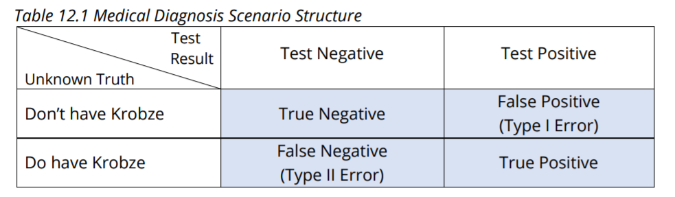
The rows show the unknown truth of not having or having Krobze, and the columns show the known negative or positive test results. The four shaded “intersection” cells show the familiar breakdown into veridical (true) results (true negative test results and true positive test results) and misleading results (Type I Error and Type II Error, which are false positive and false negative test results). As we’ll see, and unlike Frequentist statistics, Bayesian analysis makes central use of statistical assumptions about population statistic values in order to calculate probability estimates for the truth of hypotheses (something that’s considered unthinkable in Frequentist statistics!).

In particular, Bayesian analysis can be used to estimate conditional (if…then…) probabilities like:

If you test negative, then what is the probability that you really don’t have Krobze?
If you test positive, then what is the probability that you really do have Krobze?

The first involves the Test Negative column: we need to calculate the probability of a true negative divided by the sum of the probabilities of true and false negatives. The second involves the Test Positive column: we need to calculate the probability of a true positive divided by the sum of the probabilities of true and false positives. In order to calculate these, we need to know, or estimate, the probability of having the disease in general–that is, how prevalent Krobze is in the population. Notice that this is really saying that we need to know, or estimate, the population proportion, and that we will incorporate it into the heart of the Bayesian analysis (something that is not done in Frequentist statistics). We also need to know how reliable the diagnostic test is.

Listed below is this required information, which is then used to fill in Table 12.2.

1 out of 100 have Krobze, for a probability of 0.01 of having Krobze and 0.99 of not.
For the diagnostic test reliability, we are given the following information:
- For people who don’t have Krobze, 90% (0.9) test negative (true negative) and 10% (0.1) test positive (false positive)
- For people who do have Krobze, 80% (0.8) test positive (true positive) and 20% (0.2) test negative (false negative)

Notice that in addition to using the above information to fill in Table 12.2—shown in bold—another row has been added to the bottom of the Table for column sums.

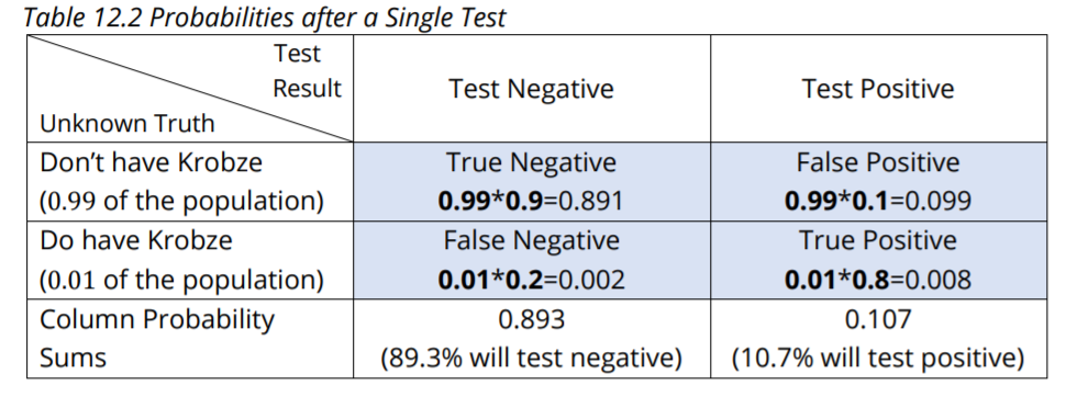
Let’s use Table 12.2 to answer the questions posed above, using Bayesian analysis.

If you test negative, what is the probability that you don’t have Krobze? This asks for the true negative rate. In jargon it’s called the specificity of the test. We use the Test Negative column. True negative/true and false negatives = 0.891/0.893 = 0.99776 which is nearly 100%.
If you test positive, what is the probability that you do have Krobze? This asks for the true positive rate. In jargon it’s called the sensitivity of the test. We use the Test Positive column. True positive/true and false positives = 0.008/0.107 = 0.074766 which is between 7% and 8%. It’s this low because Krobze is fairly rare, with only a 1% prevalence in the population, so false positives dominate the true positives.

More key Bayesian Terminology

The two Don’t & Do have Krobze cells in table 12.2 show prior probabilities.
The four shaded True False Negative Positive cells show joint probabilities.
The two Column Probability Sums cells show marginal probabilities.
The two calculated solutions 0.99776 and 0.074766 are posterior probabilities.

Many people feel that all of this makes better sense when we use frequencies rather than probabilities, so let’s do it that way too.

Consider 1,000 random people. Below are the frequencies we expect, which are then used to fill in Table 12.3.

990 won’t have Krobze (99 out of 100 don’t have it) and of those,
1. 891 (90% of 990) test negative (true negative)
2. 99 (10% of 990) test positive (false positive)
10 will have Krobze (1 out of 100 have it), and of those
1. 8 (80% of 10) test positive (true positive)
2. 2 (20% of 10) test negative (false negative)

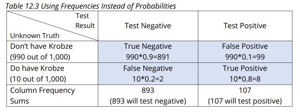
If you test negative, how likely is it that you don’t have Krobze? 891/893 = 0.99776; same as above.
If you test positive, how likely is it that you do have Krobze? 8/107 = 0.074766; same as above.

The Bayesian analysis method is especially useful because it can be used successively to update probability estimates. Let’s say you tested positive the first time and want to have another type of test (with the same diagnostic reliability) performed. Table 12.4 shows the conditions and outcomes for the second test. The posterior probability of 0.074766 based on your first positive test now becomes the prior probability for the
second test.

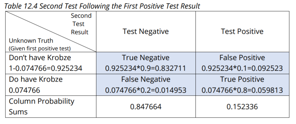
Say that you test negative the second time. The probability that you don’t have Krobze given that the second test is negative is: 0.832711/0.847664 = 0.98236; about 98%. Instead, say that you again test positive. The probability that you do have Krobze following the second positive test result is: 0.059813/0.152336 = 0.392637; about 39%.

Keep in mind that Krobze is fairly rare (1 in a 100). So, false positive test results tend to dominate the Test Positive column: that’s largely why we got 7% after the first positive test and 39% after the second positive test. Test reliability matters too, as we’ll see next.

A More Reliable Test

Let’s say that instead, the doctor orders a much more reliable (and much more expensive) test the second time. It detects both true negatives and true positives 99% of the time. Table 12.5 covers this situation.

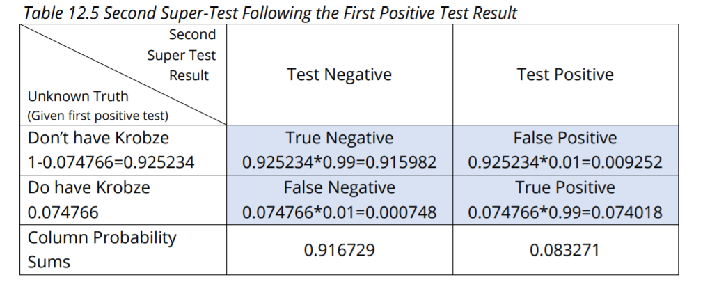
Say that you test negative the second time with the super-test. The probability that you don’t have Krobze given the first positive test result and the second negative super-test result is: 0.915982 / 0.916729 = 0.999184; nearly 100%. Finally, say that you test positive the second time with the super-test. The probability that you do have Krobze given the first positive test and the second positive super-test is: 0.074018 / 0.083271 = 0.888888; about 89%.

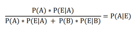
Bayesian Analysis Formulas

So far, I’ve used a table format to illustrate the application of Bayes’ Formula because I have found that people have an easier time following along than when I use the official formula. That said, I would be remiss if I didn’t show you the formula. There are several renditions of Bayes’ formula to choose from. This rendition aligns best with the table format we’ve been using.

P(A) is the prior; the prevalence of Krobze in the population (.01)
P(B) is the probability of not having Krobze in the population (1 – .01 = .99)
E is the evidence of a positive test result (corresponding to the positive test column in the table)
| is the symbol for “given that”
P(E|A) is the probability of testing positive given that you do have Krobze (0.8)
P(E|B) is the probability of testing positive given that you don’t have Krobze (0.1)
P(A|E) is what you want to know: the probability you have Krobze given that you test positive

Using again the first Krobze example when you test positive the first time, we get

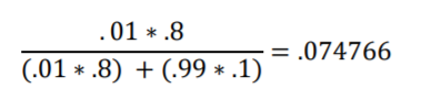
This is the same posterior probability that we got earlier using the table format.

Bayesian Analysis: A Note on Priors

With the above analyses we were extremely fortunate to know that, in general, 1 in 100 people have Krobze. That gave us our initial prior probabilities (0.01 and 0.99) which we needed to get started. What if we don’t know these initial prior probabilities? One alternative is to use expert opinion, which is somewhat subjective and may be quite incorrect. Another is to use what are called noninformative priors.

For example, if we have no idea what the initial prior probability of Krobze is, we could use the noninformative priors of equal probabilities for Don’t Have Krobze (0.5) and Have Krobze (0.5). As you can imagine, we’ll get quite different results using priors of 0.5 and 0.5 instead of 0.99 and 0.01. Determining valid priors is important, and it can be tricky. But luckily, the more data we have to update the prior with, the less important the prior becomes. Frequentist statistics does not incorporate prior probabilities into the analysis and so it doesn’t need to make assumptions about priors.

A Note on Testing Competing Hypotheses in Bayesian Analysis

Let’s say we are planning to survey Flowing Wells regarding a new public health policy and that we have two competing hypotheses. For a change of pace, we’ll use rational numbers (fractions) rather than decimal numbers. Our two competing hypotheses are H₁ that the population is 1/3 in favor and H₂ that the population is 2/3 in favor. For the prior probabilities we’ll assume equal probabilities of 1/2 that each of the hypotheses is true. Next, suppose we have a random sample of 10 survey respondents and that 4 are in favor (4/10). Based on this sample data, the Bayesian method updates the 1/2 prior probability for H₁ to the posterior probability of 4/5 and updates the 1/2 prior probability for H₂ to the posterior probability of 1/5. Given these results we’d opt for H₁ over H₂.

Since Frequentist statistics does not incorporate prior probabilities into its analysis, it never derives a probability that a given hypothesis is true.

A Note on Estimating Population Statistic Values

More sophisticated Bayesian analysis involves entire distributions. For example, let’s say we are trying to estimate a population proportion for an agree-or-disagree opinion survey question.

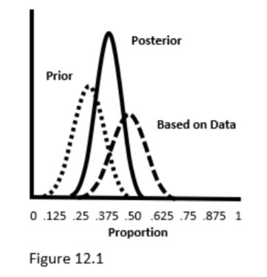
Figure 12.1 shows

1) the prior distribution for the population proportion estimate proposed by an expert,
the proportion sampling distribution based on random sample data from the population, and
the resulting posterior distribution for the population proportion estimate derived via Bayesian updating of #1 using #2.

From the posterior, we can see that the most likely estimate for the population proportion is .375. We can also determine the interval containing 95% of the posterior’s area: from .25 to .50. This is called a Bayesian credible interval, which is subtly different from a Frequentist confidence interval. Credible Interval: Given our priors and our sample data, there is a 95% chance that the population proportion falls within the 95% credible interval; valid priors and distributional assumptions need to be incorporated into the analysis.

Confidence Interval: 95% of the 95% confidence intervals derived from sample data will contain the population proportion; no priors are needed and the statistical methods themselves embody distributional assumptions (such as assuming that the z-distribution is an appropriate approximation to the binomial distribution).

You can see that Bayesian analysis leads to stronger declarations than Frequentist analysis does, but that the legitimacy of those declarations rests, in part, on the validity of the prior probabilities. Keep in mind, though, that the prior probabilities become less important as more data is used to update the probabilities. Given truly realistic priors or noninformative priors plus adequate quantities of data, Bayesian analysis becomes—for those so inclined—an attractive alternative to Frequentist statistics. Bayesian analysis is quite flexible, and it can get extraordinarily complicated. Here, we’ve taken a peek at the tip of the Bayesian iceberg.

References

J.E. Kotteman. Statistical Analysis Illustrated – Foundations .

Content for this article is published via Copyleft. You are free to copy and distribute the content of this article.