Maximum Likelihood Estimation > EM Algorithm (Expectation-maximization)
You might want to read this article first: What is Maximum Likelihood Estimation?
What is the EM Algorithm?
The Expectation-Maximization (EM) algorithm is a way to find maximum-likelihood estimates for model parameters when your data is incomplete, has missing data points, or has unobserved (hidden) latent variables. It is an iterative way to approximate the maximum likelihood function. While maximum likelihood estimation can find the “best fit” model for a set of data, it doesn’t work particularly well for incomplete data sets. The more complex EM algorithm can find model parameters even if you have missing data. It works by choosing random values for the missing data points, and using those guesses to estimate a second set of data. The new values are used to create a better guess for the first set, and the process continues until the algorithm converges on a fixed point.
See also: EM Algorithm explained in one picture.
MLE vs. EM
Although Maximum Likelihood Estimation (MLE) and EM can both find “best-fit” parameters, how they find the models are very different. MLE accumulates all of the data first and then uses that data to construct the most likely model. EM takes a guess at the parameters first—accounting for the missing data—then tweaks the model to fit the guesses and the observed data. The basic steps for the algorithm are:
- An initial guess is made for the model’s parameters and a probability distribution is created. This is sometimes called the “E-Step” for the “Expected” distribution.
- Newly observed data is fed into the model.
- The probability distribution from the E-step is tweaked to include the new data. This is sometimes called the “M-step.”
- Steps 2 through 4 are repeated until stability (i.e. a distribution that doesn’t change from the E-step to the M-step) is reached.
The EM Algorithm always improves a parameter’s estimation through this multi-step process. However, it sometimes needs a few random starts to find the best model because the algorithm can hone in on a local maxima that isn’t that close to the (optimal) global maxima. In other words, it can perform better if you force it to restart and take that “initial guess” from Step 1 over again. From all of the possible parameters, you can then choose the one with the greatest maximum likelihood.
In reality, the steps involve some pretty heavy calculus (integration) and conditional probabilities, which is beyond the scope of this article. If you need a more technical (i.e. calculus-based) breakdown of the process, I highly recommend you read Gupta and Chen’s 2010 paper.
Applications
The EM algorithm has many applications, including:
- Dis-entangling superimposed signals,
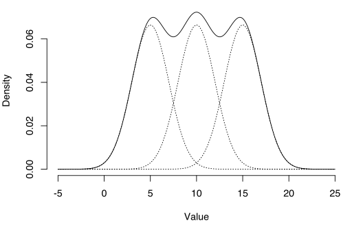
- Estimating Gaussian mixture models (GMMs),
- Estimating hidden Markov models (HMMs),
- Estimating parameters for compound Dirichlet distributions,
- Finding optimal mixtures of fixed models.
Limitations
The EM algorithm can be very slow, even on the fastest computer. It works best when you only have a small percentage of missing data and the dimensionality of the data isn’t too big. The higher the dimensionality, the slower the E-step; for data with larger dimensionality, you may find the E-step runs extremely slow as the procedure approaches a local maximum.
References:
Dempster, A., Laird, N., and Rubin, D. (1977) Maximum likelihood from incomplete data via the EM algorithm, Journal of the Royal Statistical Society. Series B (Methodological), vol. 39, no. 1, pp. 1ñ38.
Gupta, M. & Chen, Y. (2010) Theory and Use of the EM Algorithm. Foundations and Trends in Signal Processing, Vol. 4, No. 3 223–296.