T Test: Contents:
- What is a T Test?
- Assumptions
- The T Score
- T Values and P Values
- Calculating the T Test
- What is a Paired T Test (Paired Samples T Test)?
- Pros and Cons of the t-test
- History of the t-test
What is a T test?
A t-test (also called Student’s t-test) is a statistical method used to assess the difference between the means of exactly two groups. It concentrates on a single numerical variable, rather than focusing on counts or relationships among multiple variables. When analyzing the average of a sample of measurements, t-tests are the most frequently used technique for data evaluation.
A similar option is ANOVA, which is used when there are more than two groups.
There are three main types of t-test:
- Independent Samples t-test: compares the means for two groups.
- Paired sample t-test: compares means from the same group at different time periods.
- One sample t-test: tests the mean of a single group against a known mean.
Watch the video for an introduction to T-tests:
Can’t see the video? Click here to watch it on YouTube.
The t test tells you how significant the differences between group means are. It lets you know if those differences in means could have happened by chance.
The t test is usually used when data sets follow a normal distribution but you don’t know the population variance. For example, you might flip a coin 1,000 times and find the number of heads follows a normal distribution for all trials. So you can calculate the sample variance from this data, but the population variance is unknown.
Or, a drug company may want to test a new cancer drug to find out if it improves life expectancy. In an experiment, there’s always a control group (a group who are given a placebo, or “sugar pill”). So while the control group may show an average life expectancy of +5 years, the group taking the new drug might have a life expectancy of +6 years. It would seem that the drug might work. But it could be due to a fluke. To test this, researchers would use a Student’s t-test to find out if the results are repeatable for an entire population.
A t test uses a t-statistic and compares this to t-distribution values to determine if the results are statistically significant. T-tests only tell you if there is a statistically significant difference; they do not tell you how large that difference is in a standardized way. For that, researchers often report an effect size measure (such as Cohen’s d).
Note that you can only uses a t test to compare two means. If you want to compare three or more means, use an ANOVA instead. It’s technically possible to compare multiple groups via repeated t-tests if you adjust for multiple comparisons. However, using a single ANOVA (followed by post-hoc tests) is typically recommended.
Assumptions
- Normality: As noted above, t-tests typically assume that the data in each group are drawn from a normally distributed population, especially for small sample sizes. If sample sizes are large the t-test is fairly robust to departures from normality, meaning that you don’t always have to stick to the assumption of normality if your sample size is large.
- Independence (for Independent Samples T-Test): Observations in one group should not be related to observations in the other group. For example, you can use a t-test for comparing two groups of students from different classes, but you should not use an independent samples t-test to compare the means of the same group of students who take the same test twice.
- Equal Variances (for Classic Independent Samples T-Test): The standard form of the independent-samples t-test assumes equal variances in the two groups, although a variant called Welch’s t-test does not assume equal variances. In elementary statistics, you’ll usually be told in the question if you have equal variances or not. In more advanced classes, you may need to run a formal test such as Levene’s test, Brown–Forsythe test, or an F-test. Most modern statistical software will include these tests when you run an independent samples t-test, so you don’t need to check before you run the test (just make sure the assumption has been met before you draw conclusions from the output).
The T Score
The t score is a ratio between the difference between two groups and the difference within the groups.
- Larger t scores = more difference between groups.
- Smaller t score = more similarity between groups.
A t score of 3 tells you that the groups are three times as different from each other as they are within each other. So when you run a t test, bigger t-values equal a greater probability that the results are repeatable.
T-Values and P-values
How big is “big enough”? Every t-value has a p-value to go with it. A p-value from a t test is the probability that the results from your sample data occurred by chance. P-values are from 0% to 100% and are usually written as a decimal (for example, a p value of 5% is 0.05).
Low p-values indicate your data did not occur by chance. For example, a p-value of .01 means there is only a 1% probability that the results from an experiment happened by chance.
Calculating the Statistic / Test Types
There are three main types of t-test:
- An Independent Samples t-test compares the means for two groups.
- A Paired sample t-test compares means from the same group at different times (say, one year apart).
- A One sample t-test tests the mean of a single group against a known mean.
Here are the general steps to conduct a t-test (the exact steps will differ slightly depending on what type of test you are running):
- State the null and alternative hypotheses: The null hypothesis asserts that there is no difference in means between the two groups, while the alternative hypothesis claims that a difference exists.
- Choose the significance level: The significance level represents the probability of committing a Type I error, or a false positive. A common significance level is 0.05, implying a 5% chance of making a Type I error.
- Calculate the t-statistic: The t-statistic measures the difference in means between the two groups.
- Identify the critical value: The critical value is the t-statistic value that separates the regions of rejection and acceptance. It is determined by the significance level and degrees of freedom.
- Make a decision: If the t-statistic exceeds the critical value, the null hypothesis is rejected, indicating sufficient evidence to conclude a difference in means between the two groups. If the t-statistic is less than or equal to the critical value, the null hypothesis is not rejected, meaning insufficient evidence to claim a difference in means between the groups.
You can find the steps for an independent samples t test here. But you probably don’t want to calculate the test by hand (the math can get very messy. Use the following tools to calculate the t test:
- How to do a T test in Excel.
- T test in SPSS.
- T-distribution on the TI 89.
- T distribution on the TI 83.
What is a Paired T Test (Paired Samples T Test / Dependent Samples T Test)?
A paired t test (also called a correlated pairs t-test, a paired samples t test or dependent samples t test) is where you run a t test on dependent samples. Dependent samples are essentially connected — they are tests on the same person or thing. For example:
- Knee MRI costs at two different hospitals,
- Two tests on the same person before and after training,
- Two blood pressure measurements on the same person using different equipment.
Opt for the paired t-test when you have two measurements on the same item, person, or thing, or when you have two items measured under a unique condition. For instance, you might compare car safety performance in vehicle research and testing by subjecting cars from different manufacturers to the same crash tests.
In contrast, a “regular” two-sample t-test compares the means of two distinct samples. For example, you might test two separate groups of customer service associates on a business-related test or assess students from two universities on their English skills. If you take a random sample from each group separately and they have different conditions, your samples are independent, and you should run an independent samples t-test (also called between-samples and unpaired-samples).
The null hypothesis for the independent samples t-test is μ1 = μ2, assuming the means are equal. With the paired t-test, the null hypothesis states that the pairwise difference between the two tests is equal (H0: µd = 0).
To calculate a paired t-test by hand, follow these steps (I used Excel):
- Subtract each Y score from each X score.
- Sum all the values from Step 1 and set this number aside temporarily.
- Square the differences from Step 1.
- Sum all the squared differences from Step 3.
- Use the t-score formula (shown above) to calculate the t-score: t = (ΣD) / sqrt((ΣD^2 – (ΣD)^2/n) / (n-1)) where ΣD is the sum of X-Y from Step 2, ΣD^2 is the sum of the squared differences from Step 4, and n is the sample size.
- Subtract 1 from the sample size to get the degrees of freedom (e.g., 11 items, so 11 – 1 = 10).
- Find the p-value in the t-table using the degrees of freedom from Step 6. If you don’t have a specified alpha level, use 0.05 (5%).
- Compare your t-table value from Step 7 to your calculated t-value. If the calculated t-value is greater than the table value at an alpha level of .05 and the p-value is less than the alpha level (p < .05), reject the null hypothesis that there is no difference between means. Note that you can disregard the minus sign when comparing the two t-values, as ± indicates direction; the p-value remains the same for both directions.
When to Choose a Paired T Test
Choose the paired t-test if you have two measurements on the same item, person or thing. But you should also choose this test if you have two items that are being measured with a unique condition.
For example, you might be measuring car safety performance in vehicle research and testing and subject the cars to a series of crash tests. Although the manufacturers are different, you might be subjecting them to the same conditions.
With a “regular” two sample t test, you’re comparing the means for two different samples. For example, you might test two different groups of customer service associates on a business-related test or testing students from two universities on their English skills.
But if you take a random sample of each group separately and they have different conditions, your samples are independent and you should run an independent samples t test (also called between-samples and unpaired-samples). The null hypothesis for the independent samples t-test is μ1 = μ2. So it assumes the means are equal. With the paired t test, the null hypothesis is that the pairwise difference between the two tests is equal (H0: µd = 0).
Paired Samples T Test By hand
Example question: Calculate a paired t test by hand for the following data: 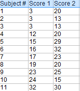
Step 1: Subtract each Y score from each X score. 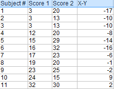
Step 2: Add up all of the values from Step 1 then set this number aside for a moment. 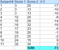
Step 3: Square the differences from Step 1. 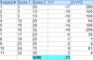
Step 4: Add up all of the squared differences from Step 3. 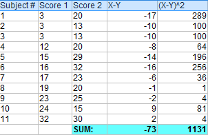
Step 5: Use the following formula to calculate the t-score: 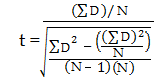
- The “ΣD” is the sum of X-Y from Step 2.
- ΣD2: Sum of the squared differences (from Step 4).
- (ΣD)2: Sum of the differences (from Step 2), squared.
If you’re unfamiliar with the Σ notation used in the t test, it basically means to “add everything up”. You may find this article useful: summation notation. 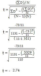
Step 6: Subtract 1 from the sample size to get the degrees of freedom. We have 11 items. So 11 – 1 = 10.
Step 7: Find the p-value in the t-table, using the degrees of freedom in Step 6. But if you don’t have a specified alpha level, use 0.05 (5%). So for this example t test problem, with df = 10, the t-value is 2.228.
Step 8: In conclusion, compare your t-table value from Step 7 (2.228) to your calculated t-value (-2.74). The calculated t-value is greater than the table value at an alpha level of .05. In addition, note that the p-value is less than the alpha level: p <.05. So we can reject the null hypothesis that there is no difference between means. However, note that you can ignore the minus sign when comparing the two t-values as ± indicates the direction; the p-value remains the same for both directions. In addition, check out our YouTube channel for more stats help and tips!
T-test pros and cons
Advantages of using Student’s t-test include:
- Simple and easy-to-use.
- Powerful for comparing means.
- Relatively inexpensive, computational wise, to conduct.
- It is not as powerful as other statistical tests, such as the ANOVA, when the sample sizes are large.
- It is sensitive to small sample sizes.
- It can be affected by outliers.
Disadvantages include:
History of the t-test
The t-test was devised by William Sealy Gosset, an English statistician employed at the Guinness Brewery in Dublin. Since his employer prohibited employees from publishing scientific papers, Gosset published his work under the pseudonym “Student.”
Gosset aimed to create a statistical test that could compare the means of two small samples, as existing tests at the time required large sample sizes, which were impractical for his work at the Guinness Brewery.
Utilizing the central limit theorem, which claims that the distribution of sample means approaches a normal distribution as the sample size grows, Gosset developed the t-test based on the assumption that the data is normally distributed.
In 1908, Gosset published his work on the t-test in the Biometrika journal. The t-test quickly gained popularity and remains widely used today.
The following are other key events in the history of the t-test: