Robust Statistics / Estimation (Robustness) & Breakdown Point

Statistics Definitions > Robust Statistics

Contents:

  1. Definition of Robust Statistics
  2. Robust & Non-Robust Estimators
  3. When You Shouldn’t Rely on Robustness
  4. Breakdown Point
  5. Sensitivity curve
  6. Robust statistics: Methods and Tests for Analysis

1. What are Robust Statistics?

Robust statistics are resistant to outliers. In other words, if your data set contains very high or very low values, then some statistics will be good estimators for population parameters, and some statistics will be poor estimators. For example, the mean is very susceptible to outliers (it’s non-robust), while the median is not affected by outliers (it’s robust).

Robust statistics give valid results under diverse conditions, even when assumptions are violated or outliers are present. The term “robust statistic” can be used to describe specific robust statistics such as the median and the interquartile range; It can also be used to describe robust statistical analyses such as robust regression. Robust statistics can also be defined as “distributionally robust and resistant to outliers” [1]. Distributionally robust means that a robust method will give us results that are reasonably close to the true value, even if data isn’t normally distributed. As such, they can be used for skewed distributions or multimodal distributions, which can be challenging to analyze with traditional statistical methods.

However, use caution when applying robust statistics to skewed or multimodal data; robust statistics can still be affected by outliers and they are not suitable for some distributions, such as mixtures of two normal distributions. In contrast, non-robust statistics are sensitive to outliers and other suboptimal conditions.

2. Robust & Non-Robust Estimators

Robust statistics are good estimators for population parameters even with outliers, while others are poor estimators. For example: The median is robust as it is not affected by outliers. Other robust statistics include:

On the other hand, the mean is non-robust as it is highly influenced by outliers. Just one high or low value can make a huge difference in its value. Other non-robust statistics include:

Robust Statistics are different from robust tests, which are defined as tests that will still work well even if one or more assumptions are altered or violated. For example, Levene’s test for equality of variances is still robust even if the assumption of normality is violated. One limitation of robust statistics is that while are resistant to outliers, we cannot use them to identify outliers or to understand why they are present in the data.

3. When You Shouldn’t Rely on Robustness.
robust statistics
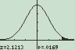
Robust statistics work on the assumption that your data follows a normal distribution.

Robust statistics assume that your underlying distribution is normal, so you shouldn’t use them for skewed or multimodal distributions. These statistics work on the assumption that the underlying data is approximately normal; if you use these statistics on a differently-shaped distribution, they will give misleading results. That said, they don’t work well for all normally shaped distributions, like mixtures of two normal distributions (called a contaminated distribution).

While robust statistics are resistant to outliers, they are not always appropriate for the same reason; it also means that the statistics you present give no idea about outliers. For example, the median house price where I live is about $250,000. That doesn’t sound too impressive, and you could be forgiven for thinking I must live in a pretty “average” town. However, I live by the river, and while most homes sell for about that price, about 1% of homes are on the river and sell for $2-3 million.

4. Breakdown Point

A breakdown point is the point after which an estimator becomes useless. It is a measure of robustness; The larger the breakdown point, the better the estimator. If an estimator has a high breakdown point, it may be called a resistant statistic. There are two types of breakdown points: finite sample breakdown points and asymptotic breakdown points.

Finite Sample Breakdown Points

The finite sample breakdown point is defined as the fraction of data which can be given arbitrary values without making the estimator, arbitrarily too large or too small. It is usually dependent on the sample size, n, and can be written as a function of n. As an example, consider the arithmetic mean as the estimator of a data set. It is given by ( x1 + x2 + … + xn )/n. You can change the calculated value of the mean by an arbitrarily large amount, simply by changing one of the data points by a large amount. Therefore, the breakdown point is just 1/n.

Asymptotic Breakdown Points

The asymptotic breakdown point is what is usually referred to when the term ‘breakdown point’ is used, and it is the finite sample breakdown point as n goes to infinity. In the example above, 1/n approaches 0 as n approaches infinity, so the (asymptotic) breakdown point of the mean is just 0. This tells us that the mean, as an estimate, is not at all robust or resistant. This is quite the opposite of the median, which has the highest possible breakdown point, of 1/2 [2].

5. Sensitivity curve and influence function

The sensitivity curve measures the effect of one outlier on the estimator. Given n – 1 fixed observations Xn − 1 = {x1, x2, . . . , xn − 1}, the sensitivity curve tells us what would happen if we add an additional observation equal to x [3]: sensitivity curve in robust statistics

For example, the sensitivity curve for the arithmetic mean is: SC(x, Tn, Xn − 1) = xn − 1.

The influence function — which does not depend on a certain set of data — is the sensitivity curve’s asymptotic counterpart. It measures the effect of a single outlier. In comparison, the breakdown point tells us how many outliers are needed to render the estimator completely useless.

The influence function is written as a function of a distribution F for an estimator T. For example, the influence function for the sample mean is T(F) = F − 1 and for the sample median the function is T(F) = F−1 (0.5).

Gross error sensitivity, which is based on the influence function, measures the maximum effect of one observation on the estimator.

While the breakdown point and influence function represents two extremes, the maxbias curve tells us what happens in the middle of these two extremes. In other words, it tells us what happens with more than one outlier but not so many that the estimator is rendered useless.

Robust statistics — methods for analysis

Robust tests still function effectively even if assumptions are altered or violated. For example, Levene’s test for equality of variances remains robust even if the assumption of normality is violated. Robust statistical analyses can give us valid results even in the absence of ideal conditions, which is typical of data that’s obtained in the field. You can have confidence in the results even if all assumptions, such as an assumption of normality, are not fully satisfied.

For example, parametric hypothesis tests, such as ANOVA and t-tests, assume a normal distribution for the data. However, these tests remain robust to deviations from normality when the sample size is sufficiently large, thanks to the central limit theorem.

Similarly, nonparametric analyses that assess the median are robust with respect to distributions since they don’t assume any specific distribution. Nonparametric analyses are resistant to the influence of outliers, in a similar way to the median.

Robust regression is designed to overcome problems associated with ordinary least squares (OLS). Outliers can skew the results of OLS regression, making it difficult to obtain accurate estimates of the slope and intercept of the line. While OLS results can be invalidated by outliers, robust regression handles them effectively.

Robust regression handles outliers in several different ways. For example:

  • Different loss function: Unlike OLS regression that minimizes the sum of squared residuals, robust regression techniques adopt alternative loss functions such as the Huber or Tukey loss functions. These functions are less sensitive to outliers.
  • Trimming or Winsorizing data: One approach is to remove or replace extreme values in the dataset. By doing so, the influence of outliers on regression results can be reduced.
  • Weighted least squares: Another approach involves assigning different weights to data points. Outliers typically have lower weights, mitigating their impact on regression results.

Robust regression can also address heteroscedasticity, which occurs when the residuals have a non-constant variance.

When performing analysis, it is important to consider the properties for the analysis is robust. For example, while traditional t-tests and ANOVAs can handle violations from the normality assumption, they are not resistant to the influence of outliers. On the other hand, nonparametric tests do not require specific distribution assumptions but assume equal dispersion across various groups in the analysis. Therefore, nonparametric tests are not robust when there are violations of the equal variances assumption.

Despite being resistant to certain assumption violations, robust statistical analyses may still be sensitive to other deviations.

Robust Tests

Robust tests, which work well even when assumptions are violated. For example, if your data violates the assumption of normality, Levene’s test for equality of variances is a robust option. This means that you can trust the results from robust tests, even if one or more assumptions have been violated.

Robust methods provide good control over the probability of a Type I error. They are not overly sensitive to small changes in a distribution, such as small departures from normality. But they also deal with much broader issues. For example [4]:

  • Curvature: In linear regression, lines as typically thought of as being straight. When a regression line has a slight curvature, this may or may not significantly affect results.
  • Heteroscedasticity (equal variances): Methods that assume homoscedasticity can be quite inaccurate in the presence of heteroscedasticity, even with large sample sizes.
  • Outliers: “Traditional” strategies for dealing with outliers, such as trimmed means or medians, are not appropriate to guard against their effects. More modern methods, such as percentile bootstrapping, help to guard against erroneously deleting important outliers.
  • Skewed distributions: The central limit theorem tells us that larger sample sizes will be approximately normal. But much larger samples may be needed than generally recognized.

References

[1] Huber P. J. 1982: Robust Statistics. Wiley, New York, p 308 [ResearchGate PDF].

[2] Wilcox, R. (2010). Fundamentals of Modern Statistical Methods: Substantially Improving Power and Accuracy. Springer Science and Business Media.

[3] Ruckstuhl, A. Half-Day 1: Introduction to Robust Estimation Techniques. Retrieved September 21, 2023 from: https://ethz.ch/content/dam/ethz/special-interest/math/statistics/sfs/Education/Advanced%20Studies%20in%20Applied%20Statistics/course-material/robust-nonlinear/robfitFolien-HT1_Druck.pdf  

[4] Wilcox, R. & Rousselet, G. A GUIDE TO ROBUST STATISTICAL METHODS IN NEUROSCIENCE. Retrieved September 22, 2023 from: https://dornsife.usc.edu/assets/sites/239/docs/CP_Wilcox_Rousselet.pdf 


Comments? Need to post a correction? Please Contact Us.