What is a Probability Density Function?
A probability density function (PDF), also called a probability density or a probability function, describes the probability distribution for a continuous random variable. It can be used to find the probability that the value of a certain event occurs within a range of values. For many continuous random variables, we can define a pdf to find probabilities of the variable falling within a range, say a and b. This probability is denoted by P (a < X < b) and is more formally given by [1]: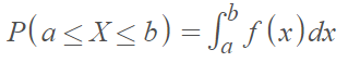
The probability that X is on the closed interval [a, b] can be calculated by integrating the pdf of the random variable X. A continuous random variable (such as one describing height, temperature, or weight) has possible values of either:
- One interval on the number line, or
- A union of disjoint intervals (“disjoint” means no points in common).
How Does It Work?
A pdf is essentially a function where its integral (the area under the curve) over an interval provides the probability of a value occurring in that interval. To put it another way, if you have two numbers – say, 120 and 140 – then you can integrate over that range to find the probability that the next IQ score you measure will fall between those two numbers. The higher the integral value is over an interval, the greater chance there is that your measured IQ score will fall somewhere within that range. In elementary statistics, we don’t usually integrate, as this involves calculus. Thankfully, most common distributions such as the normal distribution, gamma distribution and cosine distribution have known formulas for pdfs, which means that we don’t need to use calculus. We can also use tables such as the z-table to give us these values or calculators — including the TI-83 graphing calculator, and statistical software packages such as SPSS. In practical terms, pdfs help us to quantify how likely something is to happen given certain conditions. As an example, if we had data on precipitation and wanted to know when it was more likely to rain, we could fit the data to a pdf to calculate those probabilities. It isn’t always obvious which probability distribution gives us the best fit, so we often choose two or more distributions to overlay on the data and see which one fits best.Relationship between PDF, CDF and the FTC
The PDF gives us the probability of a random variable at a specific range of values, while the cumulative distribution function (CDF) gives the probability of a random variable below or equal to a specific value. For example, we could use the PDF to tell us what the probability is a baby will weigh between 8 and 9 pounds. We can use the CDF to tell us the probability a baby will weight below 8 pounds — and with a little math, we can also use the CDF to tell us the probability that the baby will weigh over 8 pounds. The pdf of a continuous random variable is also the derivative of its CDF. The Fundamental Theorem of Calculus (FTC) allows us to express the CDF, F(x), in terms of its PDF [2]: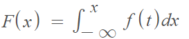 The term probability distribution function is sometimes used to mean with probability density function. For example, this paper on Hilbert Spaces describes a probability distribution function for spin quantum states. However, in the vast majority of cases, the correct term is probability density function to avoid confusion with cumulative distribution functions (CDFs).
Probability Density Function vs. Probability Mass Function
PDFs are used to define probabilities for random variable probabilities landing within a range of values, while a probability mass function (PMF) can give us probabilities for a single value. If a random variable can only have certain values (such as drawing cards from a standard deck), a PMF describes the probabilities of the outcomes. On the other hand, you would use a PDF for continuous random variables that are not restricted to a set range of distinct values: they can take on any number — including decimals and fractions — within a range. Some examples include weight, height and time. If you have continuous variables, you can’t write out every possible value because you would have infinite possibilities to write out (which is, of course, impossible). This fact is important because it tells us that the probability a continuous random variable takes on any specific value of x is zero (because 1/∞ = 0). In other words, it is not possible to calculate P(X = x) for a continuous random variable; What you can do is create a PDF; a formula that describes all possible outputs for ranges of data. A common confusion happens because although the PDF is defined for a range of values and the PMF is defined for distinct values, a calculator for a PDF will give us probabilities for single values as well. This happens because the calculator is actually calculating a tiny range behind the scenes. For example, you might type in X = 5 and get an answer of 0.02345 (2.345%). The calculator isn’t calculating the PDF at exactly X = 5, it’s calculating it for a very tiny range around that number — say from X = 4.99999 to X = 5.000001.PDF Properties
For f(x) to be a “legitimate” pdf, it must have the following properties:- f(x) ≥ 0 for all x (in other words, f(x) must be nonnegative for every value of the random variable).


Probability Density Function Examples
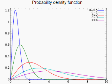
Rayleigh Distribution PDF
The notation X Rayleigh(σ) means that the random variable X has a Rayleigh distribution with shape parameter σ. The PDF (X > 0) is:Where e is Euler’s number. The distribution gets wider and flatter as σ increases.
Normal Distribution
The normal distribution (a.k.a. the “bell curve”) is defined by the pdf:Where:
- μ and σ are fixed constants.
- ex = Exponential function [3].
References
- Continuous Random Variables and Probability Distributions. Retrieved August 1, 2021 from: https://www.colorado.edu/amath/sites/default/files/attached-files/ch4_0.pdf
- 2.3 – The Probability Density Function. Retrieved August 1, 2021 from: https://blogs.ubc.ca/math105/continuous-random-variables/the-pdf/
- Kjos-Hanssen, B. (2019) Statistics for Calculus Students. Retrieved April 30, 2021 from: https://dspace.lib.hawaii.edu/handle/10790/4572