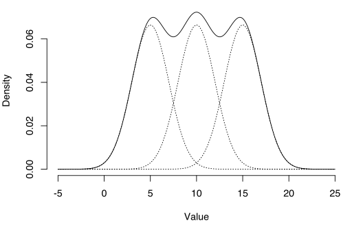
A Gaussian mixture model is a distribution assembled from weighted multivariate Gaussian* distributions. Weighting factors assign each distribution different levels of importance. The resulting model is a super-position (i.e. an overlapping) of bell-shaped curves.
Gaussian mixture models are semi-parametric. Parametric implies that the model comes from a known distribution (which is in this case, a set of normal distributions). It’s semi-parametric because more components, possibly from unknown distributions, can be added to the model.
Uses
GMMs are widely used for clustering and density estimation in physics. However they do have a wide range of applications in other fields like modeling weather observations in geoscience (Zi, 2011), certain autoregressive models, or noise from some time series.
If you think your data stems from a set of different normal distributions, then the GMM is an appropriate analysis tool. The normal distribution is an underlying assumption, which means that while it’s assumed the distributions are Gaussian, they may not be. In some cases, you may not be able to tell, but use logic or prior knowledge to assume your data has a normal distribution. Therefore, models created from a GMM methods carry with them a certain level of uncertainty. However, it’s easy to use (most popular software has the capability of producing GMMs) and — compared to non-parametric modeling — is relatively simple.
In most cases, you’ll be using software to create Gaussian mixture models. Clustering, K-means and ISODATA are based on the Gaussian mixture model.
The basic formula for a GMM with m components is:

*Note: In statistics, the Gaussian distribution is called the normal distribution or the normal curve. In the social sciences, it’s called the bell curve.
References:
Li,Z. Applications of Gaussian Mixture Model to Weather Observations. IEEE Geoscience and Remote Sensing Letters ( Volume: 8, Issue: 6, Nov. 2011 )
McLachlan, G. & Peel, D. (2000). Finite Mixture Models. Wiley-Interscience.