Statistics Definitions > Frequentist Statistics:
What are Frequentist Statistics?
Frequentist statistics (sometimes called frequentist inference) is an approach to statistics. Frequentist statistics uses formal frameworks and rules to conduct hypothesis tests and find p-values and confidence Intervals. Probability is defined as long-term frequency in a repeatable, random experiment [1]. The polar opposite is Bayesian statistics, where unknown quantities are treated probabilistically and the state of the world is seen as always updatable.
For every statistics problem, there’s data. And for every data set there’s a test with rigid formulas and rules.
For example, we might say: “If H0 is true, then we would expect to get a result as extreme as the one obtained from our sample 2.9% of the time. Since that p-value is smaller than our alpha level of 5%, we reject the null hypothesis in favor of the alternate hypothesis.”
Deviation from the rules is never allowed if you want your frequentist research to be considered statistically sound.
The four pillars of frequentist statistics
In addition to the normal distribution, three other standardized probability distributions are known as the “big four” of frequentist statistics. These are the chi-squared-distribution, t-distribution, and f-distribution. Each of these distributions is actually a family of distributions, with each family consisting of many instances of the same type of distribution [2]:
- Normal distribution: used for sample statistics related to binomials and ranks.
- T-distribution: for sample statistics related to means—such as average height of a sample of people. The t-distribution incorporates additional uncertainty into the equation. When there is no additional uncertainty, it is equivalent to the normal-distribution
- Chi-squared distribution: For sample frequentist statistics related to variances—such as the variety of heights within a sample of people.
- F-distribution: For comparing two sample variances—such as comparing the variety of heights between two samples of people.
Bayesian vs frequentist statistics
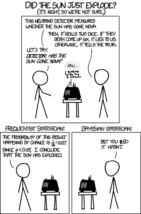
Frequentist statistics are the type of statistics you’re usually taught in your first statistics classes, like AP statistics or Elementary Statistics. You’ve got your formulas, your probabilities, and your rigid calculations. Bayesian statistics uses some of that information, but it isn’t the be-all and end all. Bayesians add prior probabilities: Has this happened before? Is it likely, based on my knowledge of the situation, that it will happen? There are a few technical differences about how each camp approaches statistics, but they aren’t very intuitive. Before I delve into the technical differences, take a look at the visual below. They probably tell you all you need to know:
Not quite there yet? How about this one (idea from George Casella’s paper Bayesians and Frequentists):  Frequentist statistics uses rigid frameworks, the type of frameworks that you learn in basic statistics, like:
For every statistics problem, there’s data. And for every data set there’s a test (and every test has its own rigid rules). The tests are based on the fact that every experiment can be repeated infinitely. Deviation from this set of rules is never allowed, and if you dare to deviate, your methods will be chided as statistically unsound. Bayesian and frequentist approaches are quite different and stem from different camps [3]:
- Frequentist: Based on work by Jerzy Neymann (1894-1981), Karl Pearson (1857 – 1936) and Abraham Wald (1902 – 1950). This relatively orthodox view of statistics tells us sampling is infinite with — usually — sharp decision rules.
- Bayesian: Based on work by Thomas Bayes (1702 – 1761), Pierre-Simon Laplace (1749 – 1827), and Bruno de Finetti (1906 – 1985). Unknown quantities are treated probabilistically and the state of the world is seen as always updatable.
Bayesian statistics is arguably more intuitive and easier to understand. Take a typical conclusion from a hypothesis test. A frequentist might say: “If H0 is true, then we would expect to get a result as extreme as the one obtained from our sample 2.9% of the time. Since that p-value is smaller than our alpha level of 5%, we reject the null hypothesis in favor of the alternate hypothesis.” On the other hand, a Bayesian might say that the odds of H0–the sun exploding tonight– are about a billion to one. Which do you find more intuitive?
The Rest of the Frequentist Statistics “Iceberg”
In addition to the normal or z-distribution, there are three other types of standardized probability distributions that form the “big four” of Frequentist statistics: the t distributions, the chi-squared -distributions, and the F-distributions. All four are highlighted below [2]. For sample statistics related to binomials and ranks we use the z-distribution, illustrated in Figure 11.1. 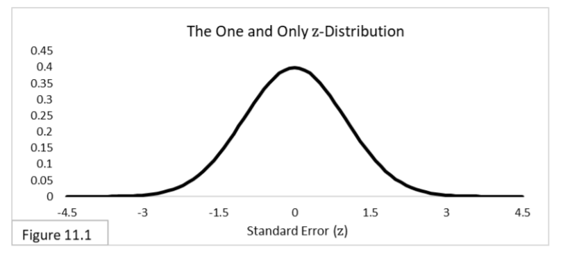
For sample statistics related to means—such as the average height of a sample of people, or the difference in average height between two samples of people—we use t-distributions, illustrated in Figure 11.2. 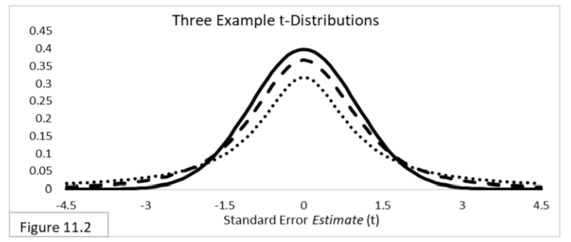 The t-distribution incorporates additional uncertainty into the equation. When there is no additional uncertainty, it is the same as the z-distribution. That’s the solid-line curve. When there is additional uncertainty, the t-distribution is more spread out, reflecting the additional uncertainty. The more additional uncertainty there is, the more spread out the t-distribution is and the wider the 95% confidence interval will be. In Figure 11.2, the dotted-line curve is the t-distribution with the most additional uncertainty of the three. For sample frequentist statistics related to variances—such as the variance (variety) of heights within a sample of people—we use chi-squared -distributions, illustrated in Figure 11.3. As you can see by the horizontal axis, chi-squared statistic values are always greater than or equal to zero.
 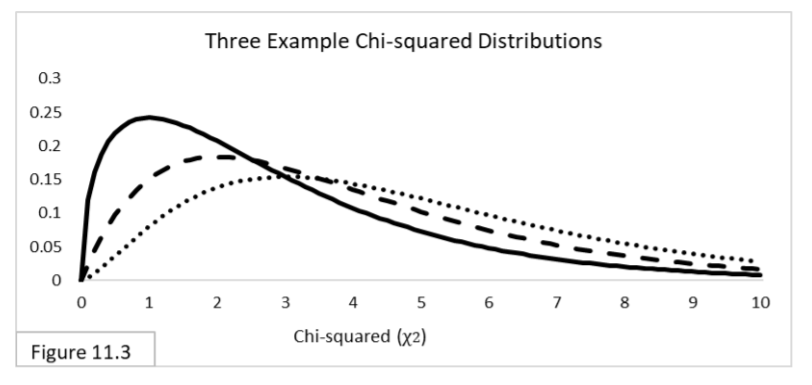 For comparing two sample variances—such as comparing the variety of heights between two samples of people—we use their ratio rather than their arithmetic difference, and we use F-distributions, illustrated in Figure 11.4. F-statistic values are also always greater than or equal to zero.
 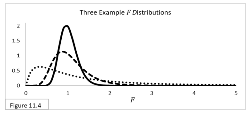 These four distributions are by far the most widely used standardized probability distributions in Frequentist statistics. For all the types of data you are likely to analyze, there are statistics that can be used to summarize that data, and those statistics can be analyzed using a standardized probability distribution. When using any of these distributions, you’ll typically reject the null hypothesis when the statistic value is located far enough out in the tail. And in all cases, assessments need to be made regarding statistical assumptions, Type I and Type II Error probabilities, statistical significance, and practical significance. Frequentist statistics has been the dominant statistical analysis methodology for over a century. However, a different methodology, with a long history itself, continues to challenge that dominance: Bayesian statistics. Next: Bayesian Analysis
References
[1] Orloff, J. & Bloom, J. The Frequentist School of Statistics. Retrieved October 25, 2023 from: https://ocw.mit.edu/courses/18-05-introduction-to-probability-and-statistics-spring-2014/8f068c9e8c401b75f9542dcf7997e542_MIT18_05S14_Reading17a.pdf [2] J.E. Kotteman. Statistical Analysis Illustrated – Foundations . Published via Copyleft. You are free to copy and distribute the content of this book. Casella, G. (undated) “Bayesians and Frequentists.” ACCP 37th Annual Meeting, Philadelphia, PA [33] [2] Casella, G. Bayesians and Frequentists: Models, Assumptions, and Inference. Retrieved October 25, 2023 from: https://archived.stat.ufl.edu/casella/Talks/BayesRefresher.pdf