Intro To Statistics > Statistical Assumptions
Previous: Binomial Approximation
Nearly all statistical tests make specific statistical assumptions about the data being analyzed. If the assumptions are not met, then the test will give questionable results and shouldn’t be used. The assumptions are often related to sample sizes and the nature of the distributions of the data values themselves. This article overviews these types of assumptions for binomials to give you a feel for what they are and why they matter.
Addressing Statistical Assumptions
In practice, the assumptions for any given statistical analysis method must be carefully assessed prior to its use. When a given method’s use cannot be justified, then a less restrictive method must be chosen—one that makes fewer or different assumptions—or the data must be transparently “massaged” in a professionally appropriate way to make it better adhere to a method’s assumptions. A professional will report everything that was done as part of any analysis.
For binomial data, the two most important assumptions have to do with sample size and extreme proportion values. Binomial sampling distributions can be approximated with the z-distribution, but only when sample sizes are large enough.
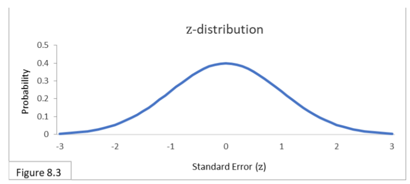
In addition, the proportion values cannot be too close to zero or one. These stipulations are critical because the formulas we’ve been using assume that the z-distribution is a proper approximation.
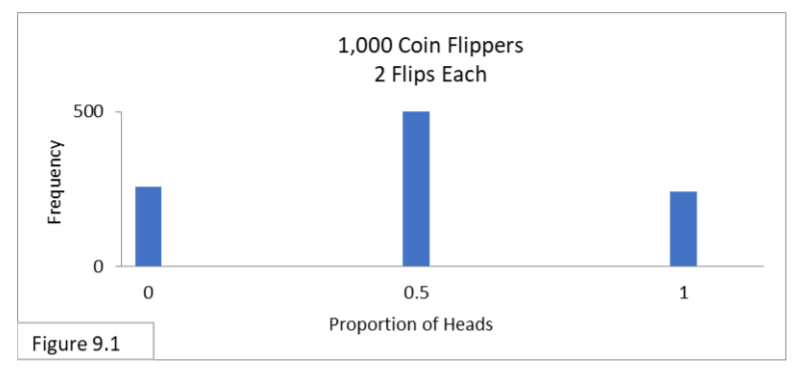
Let’s look at these issues in more detail. If the sample size is too small, the z-distribution is a poor approximation to the binomial distribution. For example, if our sample size is only 2, then the z-distribution is obviously a poor approximation as shown by the sampling distribution in this image:
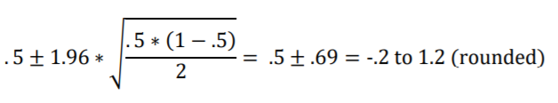
The approximation is so poor that the 95% confidence interval calculated via the formula, shown below, goes out-of-bounds on both sides with proportion boundary lines of -.2 and 1.2. These are both infeasible values for proportions!
When p is too close to zero or one, then the binomial distribution will distort from the normal bell shape. In such cases the z-distribution will also be a poor approximation.
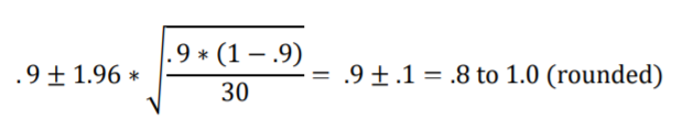
This next figure shows that the sampling distribution for p of 0.9 with sample size of 30 is distorted from the normal bell shape.
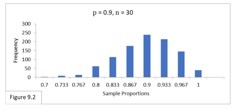
The 95% confidence interval calculated via the formula, shown below, has the extreme proportion boundary line value of 1 on the righthand side (prior to rounding, it actually calculates to slightly greater than 1).
Meeting Statistical Assumptions with a Rule of Thumb
How can we determine whether the z-distribution will be a good approximation for a given binomial sampling distribution? Both p and n influence the nature of the sampling distribution. So, the values of both n and p must be considered together. A commonly used rule-of thumb for the minimum sample size, n, needed for any given proportion, p, is to make sure n is large enough so that
n * p > 10 and n ∗ (1 − p) > 10
For Figure 9.1 (the first distribution shown above), by using this rule-of-thumb for p of 0.5 we can determine that n of 2 is too small because 2 *.5 only equals 1. On the other hand, with n of 20 we get 20 * (.5) which equals 10.
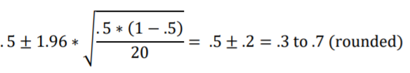
This next figure illustrates that with a sample size of 20, the sampling distribution has filled in and narrowed enough to attain a normal shape.
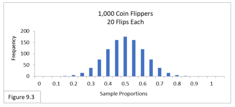
The 95% confidence interval calculated with the formula, shown below, appears to be accurate in light of Figure 9.3.
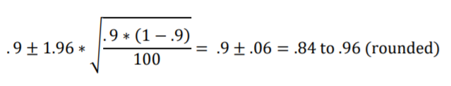
For Figure 9.2 above, by using this statistical assumptions rule-of-thumb for p of 0.9, we can determine that n of 30 is too small because 30*(1-0.9) only equals 3. On the other hand, with n of 100 we get 100 * (1 – 0.9) which equals 10. Figure 9.4 illustrates that with a sample size of 100, the sampling distribution has narrowed enough to attain a normal shape.

And the 95% confidence interval calculated with the formula, shown below, now appears to be accurate in light of Figure 9.4.
So, in summary, the z-distribution approximates the binomial distribution, and sample sizes must be adequate for the formulas to work correctly, and p cannot be too close to zero or one. With sample sizes that are too small and p that are too close to zero or one, alternatives called exact methods can be used.
For more examples, see: Normal approximation to the binomial.
You can find many more articles on the site addressing statistical assumptions for specific tests and procedures, including :
Next: Analyzing the Difference Between Two Groups Using Binomial Proportions
Author: J.E. Kotteman.
References
J.E. Kotteman. Statistical Analysis Illustrated – Foundations .
Content for this article (Statistical Assumptions) is published via Copyleft. You are free to copy and distribute the content of this article.