Contents:
What is a One Sample T Test?
The one sample t test compares the mean of your sample data to a known value. For example, you might want to know how your sample mean compares to the population mean. You should run a one sample t test when you don’t know the population standard deviation or you have a small sample size. For a full rundown on which test to use, see: T-score vs. Z-Score.
Assumptions of the test (your data should meet these requirements for the test to be valid):
- Data is independent.
- Data is collected randomly. For example, with simple random sampling.
- The data is approximately normally distributed.
One Sample T Test Example
Watch the video for an example or read the steps below:
Example question: your company wants to improve sales. Past sales data indicate that the average sale was $100 per transaction. After training your sales force, recent sales data (taken from a sample of 25 salesmen) indicates an average sale of $130, with a standard deviation of $15. Did the training work? Test your hypothesis at a 5% alpha level.
Step 1: Write your null hypothesis statement (How to state a null hypothesis). The accepted hypothesis is that there is no difference in sales, so:
H0: μ = $100.
Step 2: Write your alternate hypothesis. This is the one you’re testing in the one sample t test. You think that there is a difference (that the mean sales increased), so:
H1: μ > $100.
Step 3: Identify the following pieces of information you’ll need to calculate the test statistic. The question should give you these items:
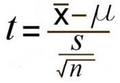
- The sample mean(x̄). This is given in the question as $130.
- The population mean(μ). Given as $100 (from past data).
- The sample standard deviation(s) = $15.
- Number of observations(n) = 25.
Step 4: Insert the items from above into the t score formula.

t = (130 – 100) / ((15 / √(25))
t = (30 / 3) = 10
This is your calculated t-value.
Step 5: Find the t-table value. You need two values to find this:
- The alpha level: given as 5% in the question.
- The degrees of freedom, which is the number of items in the sample (n) minus 1: 25 – 1 = 24.
Look up 24 degrees of freedom in the left column and 0.05 in the top row. The intersection is 1.711. This is your one-tailed critical t-value.
What this critical value means in a one tailed t test, is that we would expect most values to fall under 1.711. If our calculated t-value (from Step 4) falls within this range, the null hypothesis is likely true.
Step 5: Compare Step 4 to Step 5. The value from Step 4 does not fall into the range calculated in Step 5, so we can reject the null hypothesis. The value of 10 falls into the rejection region (the left tail).
In other words, it’s highly likely that the mean sale is greater. The one sample t test has told us that sales training was probably a success.
Want to check your work? Take a look at Daniel Soper’s calculator. Just plug in your data to get the t-statistic and critical values.
One Sample T Test in SPSS
Watch the video, which shows you how to run the test and read the results in SPSS:
References
Beyer, W. H. CRC Standard Mathematical Tables, 31st ed. Boca Raton, FL: CRC Press, pp. 536 and 571, 2002.
Agresti A. (1990) Categorical Data Analysis. John Wiley and Sons, New York.
Friedman (2015). Fundamentals of Clinical Trials 5th ed. Springer.”
Salkind, N. (2016). Statistics for People Who (Think They) Hate Statistics: Using Microsoft Excel 4th Edition.