Multidimensional Scaling: Definition, Overview, Examples

Data Analysis > Multidimensional Scaling

Contents:

What is Multidimensional Scaling?

When to Use MDS
A Simple Example
Basic steps:
Potential Pitfalls
Notation
History and Subtypes
Multidimensional scaling vs. Factor Analysis
Similar Techniques

What is Multidimensional Scaling?

Multidimensional scaling is a visual representation of distances or dissimilarities between sets of objects. “Objects” can be colors, faces, map coordinates, political persuasion, or any kind of real or conceptual stimuli (Kruskal and Wish, 1978). Objects that are more similar (or have shorter distances) are closer together on the graph than objects that are less similar (or have longer distances). As well as interpreting dissimilarities as distances on a graph, MDS can also serve as a dimension reduction technique for high-dimensional data (Buja et. al, 2007).

The term scaling comes from psychometrics, where abstract concepts (“objects”) are assigned numbers according to a rule (Trochim, 2006). For example, you may want to quantify a person’s attitude to global warming. You could assign a “1” to “doesn’t believe in global warming”, a 10 to “firmly believes in global warming” and a scale of 2 to 9 for attitudes in between. You can also think of “scaling” as the fact that you’re essentially scaling down the data (i.e. making it simpler by creating lower-dimensional data). Data that is scaled down in dimension keeps similar properties. For example, two data points that are close together in high-dimensional space will also be close together in low-dimensional space (Martinez, 2005). The “multidimensional” part is due to the fact that you aren’t limited to two dimensional graphs or data. Three-dimensional, four-dimensional and higher plots are possible.

MDS is now used over a wide variety of disciplines. It’s use isn’t limited to a specific matrix or set of data; In fact, just about any matrix can be analyzed with the technique as long as the matrix contains some type of relational data (Young, 2013). Examples of relational data include correlations, distances, multiple rating scales or similarities.

As you may be able to tell from the short discussion above, MDS is very difficult to understand unless you have a basic understanding of matrix algebra and dimensionality. If you’re new to these concept, you may want to read these articles first:
What is dimensionality?
Introduction to Matrices and Matrix Algebra.

When to Use MDS

Let’s say you were given a list of city locations, and were asked to create a map that included distances between cities. The procedure would be relatively straightforward, involving nothing more complicated than taking a ruler and measuring the distance between each city. However, what if you were given only the distances between the cities (i.e. their similarities) — and not their locations? You could still create a map — but it would involve a fair amount of geometry, and some logical deductions. Kruskal & Wish (1978) — the authors of one of the first multidimensional scaling books — state that this type of logic problem is ideal for multidimensional scaling. You’re basically given a set of differences, and the goal is to create a map that will also tell you what the original distances where and where they were located.
Back to Top

A Simple Example

Multidimensional scaling uses a square, symmetric matrix for input. The matrix shows relationships between items. For a simple example, let’s say you had a set of cities in Florida and their distances:

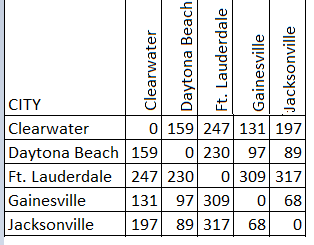
The scaling produces a graph like the one below.

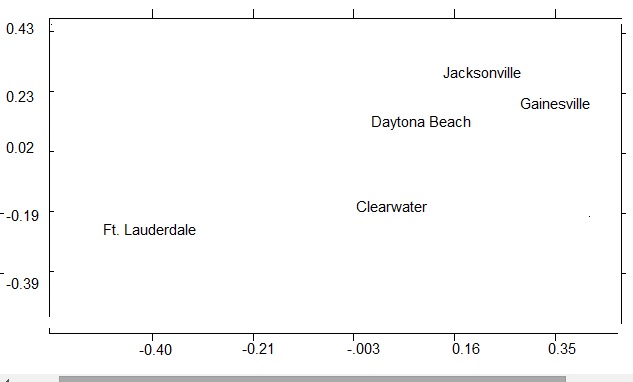
The very simple example above shows cities and distances, which are easy to visualize as a map. However, multidimensional scaling can work on “theoretically” mapped data as well. For example, Kruskal and Wish (1978) outlined how the method could be used to uncover the answers to a variety of questions about people’s viewpoints on political candidates. This could be achieved by reducing the data and issues (say, partisanship and ideology) to a two-dimensional map.
Back to Top

Basic steps:

Assign a number of points to coordinates in n-dimensional space. N-dimensional space could be 2-dimensional, 3-dimensional, or higher spaces (at least, theoretically, because 4-dimensional spaces and above are difficult to model). The orientation of the coordinate axes is arbitrary and is mostly the researcher’s choice. For maps like the one in the simple example above, axes that represent north/south and east/west make the most sense.
Calculate Euclidean distances for all pairs of points. The Euclidean distance is the “as the crow flies” straight-line distance between two points x and y in Euclidean space. It’s calculated using the Pythagorean theorem (c² = a² + b²), although it becomes somewhat more complicated for n-dimensional space (see “Euclidean Distance in n-dimensional space“). This results in the similarity matrix.
Compare the similarity matrix with the original input matrix by evaluating the stress function. Stress is a goodness-of-fit measure, based on differences between predicted and actual distances. In his original 1964 MDS paper, Kruskal wrote that fits close to zero are excellent, while anything over .2 should be considered “poor”. More recent authors suggest evaluating stress based on the quality of the distance matrix and how many objects are in that matrix.
Adjust coordinates, if necessary, to minimize stress.

Potential Pitfalls

A 2D graph, like the city distance graph above, is the easiest type of graph to figure out. However, a 2D graph might be distorted; it could also be a poor representation of similarities or distances. If this happens, you can increase the dimensionality of the graph (i.e. to a 3D graph). However, 3D and above graphs are difficult to represent on a flat computer screen or sheet of paper. Plus, they are more difficult for even the most gifted mathematician to comprehend. The goal of multidimensional scaling is to simplify a complex matrix, so anything more than a 3D graph rarely makes sense.
Back to Top

Notation

Although MDS is commonly used as a measure of dissimilarity, MDS can technically measure similarity as well. Dissimilarity between two points r and s is denoted δ_rs and similarity is denoted s_rs. Small δ_rs indicates values that are close together and larger values indicate values that are farther apart (i.e. are more dissimilar). On the other hand, similarity values are the opposite: small s_rs indicates values that are farther apart; larger values suggest more similarity (i.e. values are closer together). Similarity measures are easily converted from one to another by a monotone decreasing transformation (Buja et. al, 2007). NCSS (n.d.) gives the following formula for the transformation:

Where:

d_rs = a dissimilarity
s_rs = a similarity

Other notation you may come across:

i and j = sometimes used in place of s and r to indicate primary and secondary points.
Δ = the matrix (usually n x n) representing the dissimilarities.
d_rs = the distance between point r and point s (not to be confused with the dissimilarity notation d_rs in the above conversion equation).
X = the matrix of coordinate values in lower-dimensional space .

History and Subtypes

boyden 1933 — Relationships of several biological species from Boyden (1933).

The term metric multidimensional scaling made its first appearance in 1938 in Richardson’s Multidimensional Psychophysics. Several people before Richardson, including Boyden (1933), had used the concept, although they didn’t call it multidimensional scaling. Boyden, a biologist, used the technique to create models for relationships between common amphibia.
Thirty years after Richardson’s work, Torgerson (1958) rediscovered and extended the method for metric MDS. The first mention of nonmetric MDS was in 1964 by Hays (in Coombs, 1964:444), who used ranks instead of distances. Thus, MDS can be divided into two sub-types, which differ in the way the dissimilarities δ_rs are transformed into distances d_rs (Cox and Cox, 2001):

Metric Multidimensional scaling, for quantitative similarities. The function f(·) defines the MDS model. Martinez (2005) states that most metric MDS methods satisfy the following equation: d_rs = f(;δ_rs). Many other function variations are possible, but they all form a linear relationship. In other words, if you double δ, you also double d (Kruskal & Wish, 1978).
Nonmetric Multidimensional scaling (also called ordinal MDS) uses qualitative similarities. Distances in ordinal MDS are on an ordinal scale. The ranks are the only reliable source of data in nonmetric MDS; distances in X are ordered “…as closely as possible as the proximities” (Borg et. al, 2012, p.37). While metric MDS shows a linear relationship, nonmetric MDS is described by a set of curves that depend only on the value of the ranks. The curve may be simple, or it may have a dozen different bumps and swerves, but they all form a rising (or falling) trend from left to right. Unlike in metric MDS, f is defined implicitly.

Choosing between the two (metric vs. nonmetric) isn’t as simple as it might seem, because

“…the several varieties of metric scaling differ from each other as much as they do from nonmetric scaling. Furthermore, it is possible…to blend metric and nonmetric scaling in a “special combination. ~ Kruskal and Wish, 1978”

According to Kruskal and Wish, the simple answer is that your choice will be limited by which computer program you’re using.

Multidimensional scaling vs. Factor Analysis

Both Multidimensional scaling (MDS) and Factor Analysis (FA) uncover hidden patterns or relationships in data. Both techniques require a matrix of measures of associations. However, while FA requires metric data, MDS can handle both metric and non metric data.

MDS is more useful than FA if you are able to create a 2D map, as you’ll be able to visually confirm your findings.
Back to Top

Similar Techniques

Multidimensional scaling is similar to Principal Components Analysis (PCA) and dendrograms. All are tools to visualize relationships, but they differ in how the data is presented. In some cases, MDS can be used as an alternative to a dendrogram. However, unlike dendrograms, MDS is not plotted in “clusters,” nor are they hierarchical structures. PCA is another similar tool, but while MDS uses a similarity matrix to plot the graph, PCA uses the original data.

Check out our YouTube channel for hundreds of statistics and probability videos!

Recommended Reading and References