Intro To Statistics > Binomial Approximation
Previous: The Limited Meaning of Statistical Significance
Binomial Approximation with the Z-Distribution
The z-distribution is important because it is the ultimate source of many of the formulas used in statistics. The sampling distributions for binomial variables are discrete distributions (discrete values such as 0, .01, .02, …, 1 on the horizontal axis and discrete frequency counts on the vertical axis), but the equation we’ll see in a moment defines a continuous distribution (continuous values on the real number line for both the horizontal and vertical axes).
Let’s transform a discrete binomial distribution to the Standard Error scale, and then to the continuous Standard Normal distribution, which is most often called the z-distribution.
First, on the horizontal axis we simply subtract .5 from each value (to center the distribution on zero) and divide each by the Standard Error determined using the below formula:
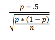
Voila, we get Figure 8.2.
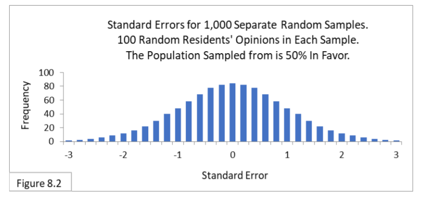
Next, we connect the tops of all the bars to make a continuous distribution, and we replace the frequency scale on the vertical axis with a probability scale (more on this below). Voila, we get Figure 8.3, the famous z-distribution. The letter z denotes the Standard Error scale.
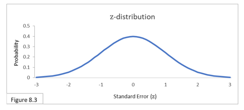
The scale on the vertical axis in Figure 8.3 is now probability. Probability is a continuous scale going from 0 to 1. A probability of 1 means something will always happen and a probability of 0 means something will never happen. A probability of 0.5 means something will happen half the time.
The z-distribution is a probability distribution that is normal, standardized, and continuous. It is one of the most important standardized probability distributions in statistics, and not just for binomial approximation. Since it’s a probability distribution, the entire area under the curve is 1. And, since it is a continuous function, probabilities for specific values—such the probability of z exactly equaling 1.96—are zero. We always need to refer to the probability of ranges—such as the probability that z is less than -1.96 or greater than 1.96.
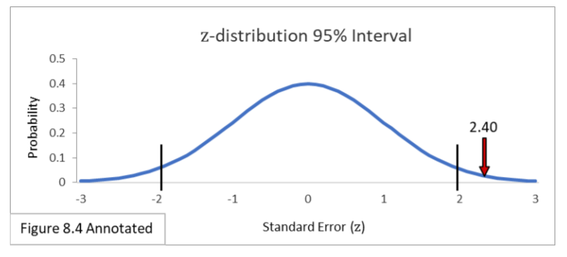
The boundary lines for the 95% interval on the Standard Normal Distribution are always -1.96 and 1.96, as shown in Figure 8.4.
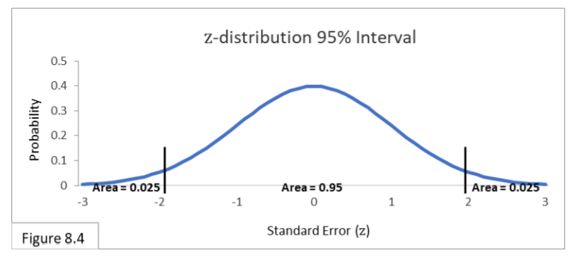
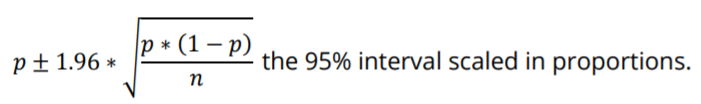
The area under the curve within the boundary lines is 0.95 and the total area outside is 0.05, with 0.025 on each side. There are two primary formulas to use for the z-distribution and standard error scale In the below formula, multiplying +1.96 times the Standard Error gives us the 95% interval expressed in proportions.
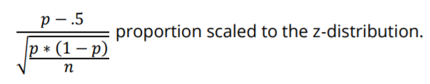
And in the below formula, dividing the difference between a proportion and a fixed proportion value (such as .5) by Standard Error gives us the difference expressed in Standard Errors.
Many statistical formulas are, or involve, such scale conversions. Let’s go through complementary examples.
Examples of Scale Conversions
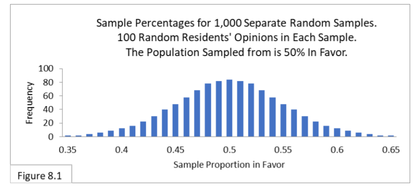
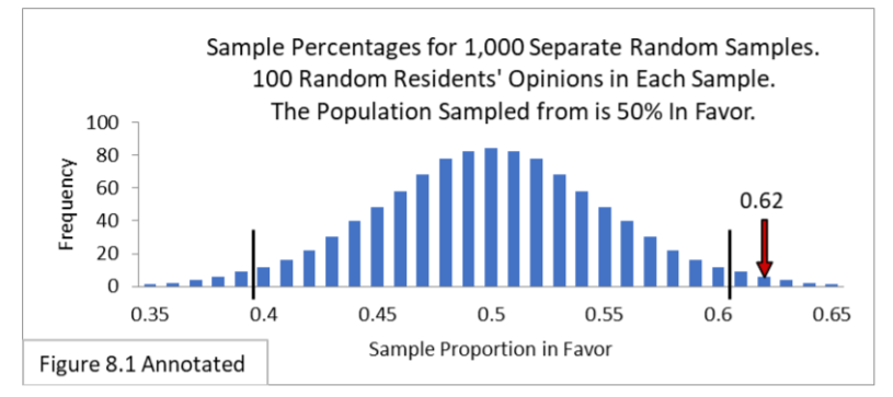
As examples of using each of the two formulas for binomial approximation, with illustrations, let’s say we took a random sample of 100 and got a sample proportion of 0.62. Our hypothesis is that the population proportion is 0.50. The 95% interval calculation gives us
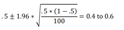
Figure 8.1, annotated below, shows the sampling distribution along with the confidence interval of 0.4 to 0.6 and the sample proportion value of 0.62 superimposed on it.
Using the second formula we get
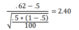
Figure 8.4, annotated below, shows the z-distribution along with its standard confidence interval of -1.96 to 1.96 and the Standard Error value of 2.40 superimposed on it.
This illustrates the equivalence between the two: the statistical result is outside the 95% interval in the same relative location. You get the same result whether you
- Calculate the confidence interval boundaries in terms of proportions using the zdistribution’s +1.96 multiplier, and then see if your sample proportion value is outside the interval, or
- calculate the Standard Error for your sample proportion, and then see if the Standard Error value is outside the z-distribution’s standard ±1.96 interval.
From here on, we’ll be using both types of calculation and illustration. The z-distribution can be used for binomial approximation. It is not an exact match, because the binomial is a discrete distribution, but, as long as the sample size is large enough, it is a very useful approximation. (There are some exceptions. See Statistical Assumptions).
Note: The equation for the continuous z-distribution curve itself is shown below. There is no practical need for you to know this equation. I put it here so you could see that there is indeed an equation that defines the z-distribution curve.
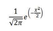
where, x is Standard Error (the horizontal axis).
For those of you acquainted with calculus, you know that you can find the area under specific regions of the curve using integration to determine the probability of having values within those regions.
Next: Statistical Assumptions
Author: J.E. Kotteman.
References
J.E. Kotteman. Statistical Analysis Illustrated – Foundations .
Content for this article is published via Copyleft. You are free to copy and distribute the content of this article.