Intro to Statistics > Statistics Case Studies
Previous: Type I & Type II Errors.
The following six short statistics case studies explore Type I Error and Type II Error under various circumstances. The odd numbered cases concentrate on Type I Error. These cases illustrate that the expected frequency of Type I Error does not change across the various circumstances. The even numbered cases concentrate on Type II Error and illustrate that the expected frequency of Type II Error does change across the various circumstances. Keep in mind that for all these cases we, being know-it-alls, know what the actual population percentages are, but the surveyors do not!
Statistics Case Studies #1
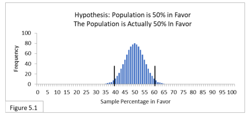
Referring to Figure 5.1, suppose a population is 50% in favor of a new public health policy, and 1,000 surveyors survey the population using random sampling of sample size 100. All 1,000 surveyors hypothesize that the population is 50% in favor, and they use the appropriate 95% confidence interval spanning from 40% to 60%. Expect 95% (within the interval) to not reject the hypothesis. They don’t know it, but they are in fact correct. Expect 5% (outside the interval) to reject the null hypothesis and so suffer a Type I Error. They don’t know it, but they are in fact
incorrect. They just happened to get a misleading random sample. Type II is irrelevant because the hypothesis is in fact correct (unbeknownst to any of the surveyors).
Now imagine that you are one of those surveyors. There’s a 95% chance that you’re one of the ones whose random sample led you to the correct conclusion, and a 5% chance that you’re one of the ones whose random sample led you to the incorrect conclusion (Type I Error).
Statistics Case Studies: Case 2
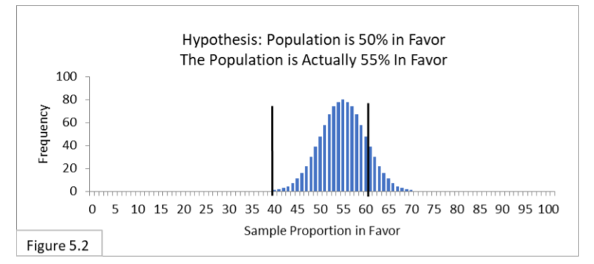
Referring to Figure 5.2, suppose a population is 55% in favor of a new public health policy, and 1,000 surveyors survey the population using random sampling of sample size 100. All 1,000 surveyors hypothesize that the population is 50% in favor and use the appropriate 95% confidence interval spanning from 40% to 60%. Expect about 85% (within the interval) to not reject the hypothesis and so suffer Type II Error. They don’t know it, but they are in fact incorrect. Expect about 15% (outside the interval) to reject the hypothesis. They don’t know it, but they are in fact correct.
Type I Error is irrelevant because the hypothesis is in fact incorrect (unbeknownst to any of the surveyors). It may seem shocking, but because 55% is so close to 50% and because 100 is a somewhat small sample size, about 85% of the surveyors are expected to reach the wrong conclusion!
Now imagine that you are one of those surveyors. There’s a 15% chance that you’re one of the ones whose random sample led you to the correct conclusion, and an 85% chance that you’re one of the ones whose random sample led you to the incorrect conclusion (Type II Error).
Case 3
Let’s increase the sample size.
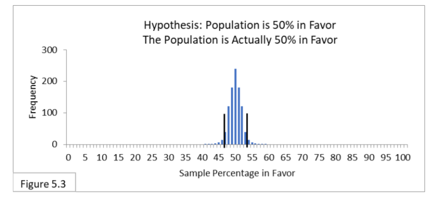
Referring to Figure 5.3, suppose a population is 50% in favor of a new public health policy, and 1,000 surveyors survey the population using random sampling of sample size 1000. All 1,000 surveyors hypothesize that the population is 50% in favor. Nothing has changed regarding Type I Error because they’re all still using a 95% interval, which now spans from 47% to 53%, and the hypothesis is true. We still expect 95% to be correct and 5% to be incorrect. Type II Error is irrelevant because the hypothesis is actually true. Now imagine that you are one of those surveyors. There’s a 95% chance that you’re one of the ones whose random sample led you to the correct conclusion, and a 5% chance that you’re one of the ones whose random sample led you to the incorrect conclusion (Type I Error).
Statistics Case Studies: Case 4
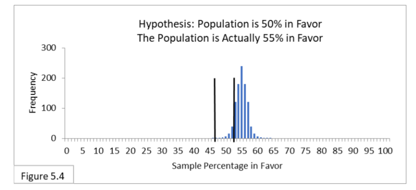
Referring to Figure 5.4, suppose a population is 55% in favor of a new public health policy, and 1,000 surveyors survey the population using random sampling of sample size 1000. Their hypothesis is that the population is 50% in favor of the new policy, and they use the corresponding 95% interval of 47%-to-53%. Because of the increased sample size—increased power—we now expect about 90% of the surveyors to be correct (rather than 15% in Case 2). And we expect about 10% to be incorrect and suffer Type II Error (rather than 85% in Case 2). That’s much better. Type I Error is irrelevant because the hypothesis is actually false. Now imagine that you are one of those surveyors. There’s a 90% chance that you’re one of the ones whose random sample led you to the correct conclusion, and a 10% chance that you’re one of the ones whose random sample led you to the
incorrect conclusion (Type II Error). Much better odds than in Case 2!
Case 5
Let’s make our Type I Error criterion stricter. Type I Error is feared more than Type II Error, and since we’ve managed, in Case 4, to lower the expected Type II Error rate to about 10%, let’s take advantage of that and make our Type I Error criterion stricter, knowing full well that will increase the likelihood of Type II Error.
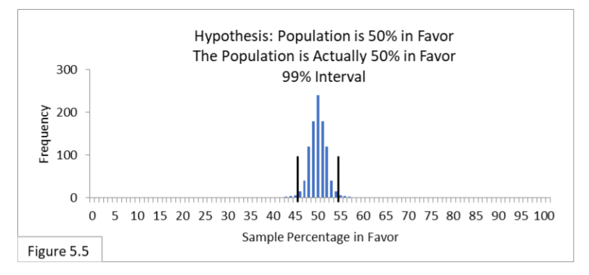
Referring to Figure 5.5, suppose a population is 50% in favor of a new public health policy, and 1,000 surveyors survey the population using random sampling of sample size 1000. Their hypothesis is that the population is 50% in favor of the new policy. Now they are going to use 99% intervals, which span from 46% to 54%. Now we expect 99% of the surveyors to be correct and 1% to be incorrect. Type II Error is irrelevant.
Now imagine that you are one of those surveyors. There’s a 99% chance that you’re one of the ones whose random sample led you to the correct conclusion, and a 1% chance that you’re one of the ones whose random sample led you to the incorrect conclusion (Type I Error).
Statistics Case Studies: Case 6
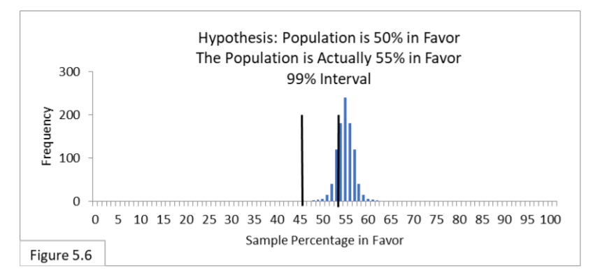
Referring to Figure 5.6, suppose a population is 55% in favor of a new public health policy, and 1,000 surveyors survey the population using random sampling of sample size 1000. Their hypothesis is that the population is 50% in favor of the new policy, and they use the corresponding 99% interval of 46%-to-54%. Because of the stricter Type I Error criterion and its wider 99% interval, we now expect about 70% of the surveyors to be correct (rather than 90% in Case 4). And we expect about 30% to be incorrect and suffer Type II Error (rather than 10% in Case 4). Type I
Error is irrelevant.
Now imagine that you are one of those surveyors. There’s a 70% chance that you’re one of the ones whose random sample led you to the correct conclusion, and a 30% chance that you’re one of the ones whose random sample led you to the incorrect conclusion (Type II Error). With sample size 1000, which would you choose, the Type I and II Errors rates of 5% and 10% as in Cases 3 and 4, or 1% and 30% as in Cases 5 and 6? Well, that depends on how costly making each kind of error is. And that depends on context. If the repercussions of Type I Error are much worse than those of Type II Error, then you’d pick 1% and 30%. If not, you’d pick 5% and 10%. Or, you could pay to have even larger samples gathered and try for 1% and 10% to get the best of both! (But remember, we’ve only considered Type II Error in cases where the population is 55% in favor. If we considered 51% to 54% we would see more Type II Error and if we considered 56% or more we would see less Type II Error.)
The Bottom Line: Sample size is an important way to manage error rates. Larger sample sizes in statistics case studies allow you to make your Type I Error level stricter, if desired, while also making sure your Type II Error level remains reasonable.
Terminology and Notation for Statistics Case Studies: Mathematically, the probability of Type I Error is denoted by the lower-case Greek letter alpha, α. The percentage level for confidence—which we’ve been referring to a lot—is (1 – α) * 100%. So, an alpha-level of 0.05 is equivalent to a confidence level of 95%. The probability of Type II Error is denoted by the lower-case Greek letter beta, β. Statistical Power is 1 – β (not made into a percentage).
So, for example, a beta level of 0.20 is equivalent to a power level of 0.80.
Next: The Central Hypothesis
References
J.E. Kotteman. Statistical Analysis Illustrated – Foundations . Published via Copyleft. You are free to copy and distribute the content of this article.