KPSS Test: Definition and Interpretation

What is the KPSS Test?

The Kwiatkowski–Phillips–Schmidt–Shin (KPSS) test figures out if a time series is stationary around a mean or linear trend, or is non-stationary due to a unit root. A stationary time series is one where statistical properties — like the mean and variance — are constant over time.

The null hypothesis for the test is that the data is stationary.
The alternate hypothesis for the test is that the data is not stationary.

Overview of How The Test is Run

The KPSS test is based on linear regression. It breaks up a series into three parts: a deterministic trend (βt), a random walk (r_t), and a stationary error (ε_t), with the regression equation:

x_t = r_t + βt + ε₁.

If the data is stationary, it will have a fixed element for an intercept or the series will be stationary around a fixed level (Wang, p.33). The test uses OLS find the equation, which differs slightly depending on whether you want to test for level stationarity or trend stationarity (Kocenda & Cerný). A simplified version, without the time trend component, is used to test level stationarity.

Data is normally log-transformed before running the KPSS test, to turn any exponential trends into linear ones.

Running the KPSS Test

Note: At the time of writing, SPSS doesn’t have an option for this test.

In R: kpss.test(x, null = c(“Level”, “Trend”), lshort = TRUE)
Where:

x is a numeric vector or univariate time series,
null is either “Level” or “Trend” (you can specify just “L” or “T”).
lshort indicates if the short version (TRUE) or long version (FALSE) should be used.

Full details can be found in the r documentation.

In Stata:
^kpss^ varname [^if^ exp] [^in^ range] [^,^ ^m^axlag^(^#^)^ ^notrend^ ]
Note: You must ^tsset^ your data before using ^kpss^; see help @tsset@ or the full Stata description for the command here.

Interpreting the Results

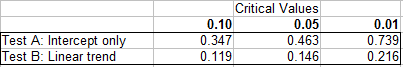
The KPSS test authors derived one-sided LM statistics for the test. If the LM statistic is greater than the critical value (given in the table below for alpha levels of 10%, 5% and 1%), then the null hypothesis is rejected; the series is non-stationary.

You can also look at the p-value returned by the test and compare it to your chosen alpha level. For example, a p-value of 0.02 (2%) would cause the null hypothesis to be rejected at an alpha level of 0.05 (5%).

Cautions

A major disadvantage for the KPSS test is that it has a high rate of Type I errors (it tends to reject the null hypothesis too often). If attempts are made to control these errors (by having larger p-values), then that negatively impacts the test’s power.
One way to deal with the potential for high Type I errors is to combine the KPSS with an ADF test. If the result from both tests suggests that the time series in stationary, then it probably is.

References:
Kocenda, E. & Cerný, A. (2017). Elements of Time Series Econometrics: An Applied Approach. Karolinum Press.
Kwiatowski et. al (1992). Testing the null hypothesis of stationarity against the alternative of a unit root. Journal of Econometrics 54 159-178. Retrieved November 22, 2106 from http://debis.deu.edu.tr/userweb/onder.hanedar/dosyalar/kpss.pdf
Wang, W. (2006). Stochasticity, Nonlinearity and Forecasting of Streamflow Processes.