Lagrange Multiplier & Constraint
A Lagrange multiplier is a way to find maximums or minimums of a multivariate function with a constraint. The constraint restricts the function to a smaller subset.
Most real-life functions are subject to constraints. For example:
- Maximizing profits for your business by advertising to as many people as possible comes with budget constraints.
- Motion of a particle usually has a distance constraint. For example, that it moves exactly 1 nanometer from a given point.
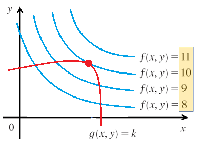
Another way to look at a constraint is that it quantifies interactions between systems. To look at this graphically, let suppose you have two functions:
- A function that you want to find a maximum or minimum for: a = f (x, y)
- A constraint g(x, y) = c.

The red dot on the graph shows the maximum of the function, given the constraints. The maximum point is where the tangent lines of both functions are equal, which in turn means that the gradient vectors are parallel. More specifically, the maximum (or minimum) of the function occurs when the gradient of the function (Δ f) equals some scalar multiple (λ) multiplied by the gradient of another function (Δ g).
How to Solve a Lagrange Multiplier Problem
While there are many ways you can tackle solving a Lagrange multiplier problem, a good approach is (Osborne, 2020):
- Eliminate the Lagrange multiplier (λ) using the two equations,
- Solve for the variables (e.g. x, y) by combining the result from Step 1 with the constraint. This gives the critical points.
- Find the largest or smallest values of the function, evaluated at the critical points.
Example Problems
Watch the video for several examples, starting with a fairly easy to follow example of minimizing the function f(x, y) = 3x + 4y, with the constraint that x2 + y2 = 100.
Advantages and Disadvantages
Although the Lagrange multiplier is a very useful tool, it does come with a large downside: while solving partial derivatives is fairly straightforward, three variables can be bit daunting (and a lot to keep track of) unless you are very comfortable with calculus. A better option is to use software, like MATLAB or R. However, most software has a steep learning curve—especially for non-programmers.
In addition, a solution for a Lagrange multiplier problem doesn’t tell you if you have a local or a global extreme (for example a global maximum or a local maximum). In order to show that the min or max is local, you have to take a couple of extra steps and show that:
- The optimization problem has
- an objective function and
- constraint functions
that are both differentiable, continuous functions,
- The problem satisfies a constraint qualification.
The constraint qualification is rather technical, but The University of Delaware’s MArco Montes (2020) gives an excellent overview of the process in handout
References
Lagrange Multiplier (PPT). Retrieved September 7, 2020 from: http://www.math.iit.edu/~rellis/teaching/152S12/inclass/Calculus%207e%20PPT%20lecture%20slides/StewartCalc7e_14_08.ppt
Montez, M. (2020). MATH529 Fundamentals of Optimization Constrained Optimization IV. Retrieved September 8, 2020 from: http://montes-de-oca.com/teaching/UD/S14-MATH529-10/Session13/handout.pdf
Nelson, S. & Nelson, E. (2014). Excel Data Analysis For Dummies. Wiley.
Osborne, J. (2020). Lagrange Multipliers. Retrieved September 7, 2020 from: http://math.bu.edu/people/josborne/MA225and230/MA230/notes/ConstrainedOptimizationNotes.pdf