Intro to Statistics > Binomial Proportions
Previous: Statistical Assumptions
Analyzing the Difference Between Two Groups Using Binomial Proportions
So far in Intro to Statistics, we’ve covered many essential foundations. Let’s put them into action while looking at another common type of analysis involving binomial proportions. We are surveying the population in Flowing Wells, but we’ll compare them to the population in a neighboring town, Artesian Wells. The reason for our surveys is to assess how residents feel about a newly proposed state government initiative.
The state government is considering state tax increases to fund some new government programs. We’re going to survey Flowing Wells residents as we have been doing, but we’re also going to survey residents in the nearby town of Artesian Wells. Historically, the town of Flowing Wells is known to lean socialist and probably favors the new taxes and programs, but the town of Artesian Wells is thought to lean libertarian and probably doesn’t. The survey is going to be conducted in each of the two towns to see if the proportions of residents that are in favor of the new taxes and programs are different in the two towns.
The corresponding Null Hypothesis is that they are not different: There is no difference between the Flowing Wells and the Artesian Wells communities’ population proportions. That is, the difference between the Flowing Wells and the Artesian Wells population proportions equals zero.
The relevant sample statistic is the Flowing Wells’ sample proportion minus the Artesian Wells’ sample proportion. (Using the Artesian Wells’ sample proportion minus the Flowing Wells’ sample proportion will give us fundamentally the same results.)
Unfortunately, the not-for-profit organization that is conducting the survey only has resources to survey 100 random residents in each town. First, let’s get a “bird’s eye view” of the situation. The Null Hypothesis is that there’s no difference between the Flowing Wells and the Artesian Wells communities’ population proportions, so let’s look at simulation results that assume that is true.
Binomial Proportions: Simulation Results
We’ll assume that both Flowing Wells and Artesian Wells have an overall community population opinion of 50% (0.50) agree, such that the difference in the population proportions equals zero. If 100 people are randomly surveyed in each of the two communities, how likely is it that various sample proportion differences could arise by chance, due to the randomness inherent in the sampling? The simulation takes two random samples of size 100 from populations that are 50%-in-favor and subtracts one of the sample proportions from the other. It does this over and over and over.
Figure 10.1 illustrates the simulation results, which is the sampling distribution of what to expect when the Null Hypothesis is true.
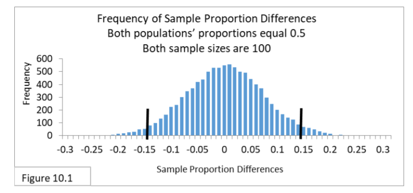
You can see that the sampling distribution for the difference between two sample proportions is a normal distribution. And it appears the 95% interval for this situation has boundary lines of -.14 and .14. So, if the difference between two sample proportions is within the interval -.14 to .14, then we won’t reject the Null Hypothesis. If it’s outside the interval, then we will reject the Null Hypothesis and say that the difference between the two communities is statistically significant. The limited resources that have constrained the sample sizes to 100 gives a fairly wide interval, where the two sample proportions have to be at least 0.15 apart to reject the Null Hypothesis. The small samples and wide confidence interval raise concerns about Type II Error.
The Standard Error formula for the difference between two population proportions is
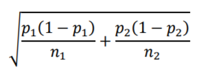
Notice that the terms within the square root follow the same “variance divided by sample size” structure we saw with the Standard Error for a single proportion. Now there is a term for each of the two populations. Both samples are size 100, and we are assuming both have population p equal to .5, making their difference equal to zero. Using the 95% confidence interval formula we get
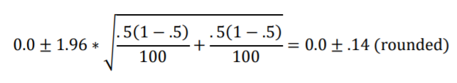
That agrees with Figure 10.1; the sampling distribution is approximated nicely by the z-distribution that’s embodied in the formula.
For an example analysis, let’s suppose the sample binomials proportions for the survey are: Flowing Wells = .52 and Artesian Wells = .44. The difference is .08, which is within the 95% interval. Conclusion: Do not reject the Null Hypothesis. (We never accept the Null Hypothesis, we just don’t reject it.)
Conducting the Survey for Binomial Proportions
Now that we’ve looked at the bird’s eye view, let’s get back to conducting the surveys. The first survey is conducted in March. We are going to analyze the survey data using the other primary formula type we’ve been utilizing. We’ll convert a sample proportion difference to the Standard Error scale. Below is the formula for the Standard Error of the difference between two sample proportions.
̂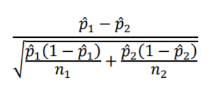
Let’s suppose the survey data yields a sample proportion for Flowing Wells of .52 and for Artesian Wells of .44. Are these two sample proportions far enough apart that we can say the difference is statistically significant? First, we’ll calculate the Standard Error of the sample proportion difference.
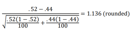
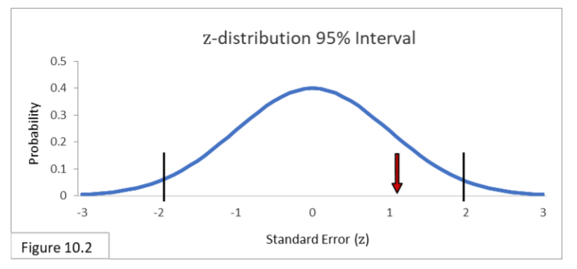
The proportion difference of .08 (.52-.44) equates to 1.136 Standard Errors. Looking now at the Standard Normal Distribution (z-distribution) in Figure 10.2 we can see that the result is inside the 95% interval and so we do not reject the Null Hypothesis that Flowing Wells and Artesian Wells have equal population proportions. The .08 sample proportion difference is not statistically significant.
Someone from the not-for-profit organization raises the issue of practical significance and suggests that 52% and 44% are different enough to be considered politically meaningful. Wait! you say. Without statistical significance we really shouldn’t even be thinking about that! The results do not allow us to talk as if the population proportions are different at all! Nonetheless, you add helpfully, with the small sample sizes, Type II Error does seem like a real possibility.
Suppose the survey is conducted again a month later, in April, and the two sample binomial proportions are farther apart: .52 and .34.
First off, since .34 is closer to zero than most of the proportions we’ve encountered so far, let’s check a statistical assumption rule-of-thumb:
n ∗ p ≥ 10 and n ∗ (1 − p) ≥ 10
With a sample size of 100 and proportion of .34 we get
100 ∗ .34 = 34 ≥ 10 and 100 ∗ (1 − .34) = 66 ≥ 10
This assumption is met comfortably, so we’ll calculate the Standard Errors of the difference between .52 and .34 and then check it with the z-distribution.
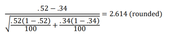
Looking at Figure 10.3 we see that 2.614 Standard Errors is outside the 95% interval.
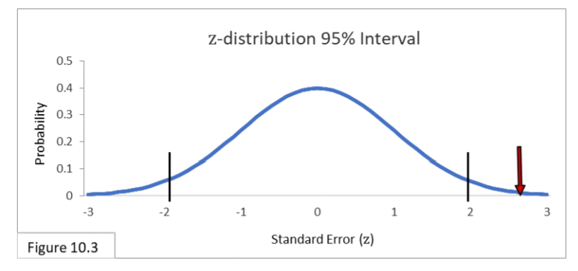
The .18 difference between .52 and .34 is statistically significant, and we do reject the Null Hypothesis that Flowing Wells and Artesian Wells have equal population proportions. Plus, it does seem that 52% and 34% are different enough to claim practical significance—that the difference has meaningful political implications.
Next, let’s say that for the following month’s survey, in May, additional resources are committed so that larger samples can be gathered. The sample statistic values are the same as two months ago, in March—sample proportions of .52 and .44— but now the sample sizes are 1000.
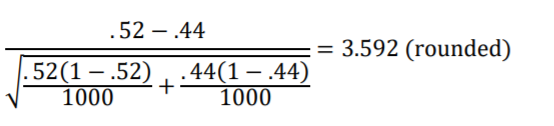
Looking at Figure 10.4 we see that 3.592 Standard Errors is outside the 95% interval.
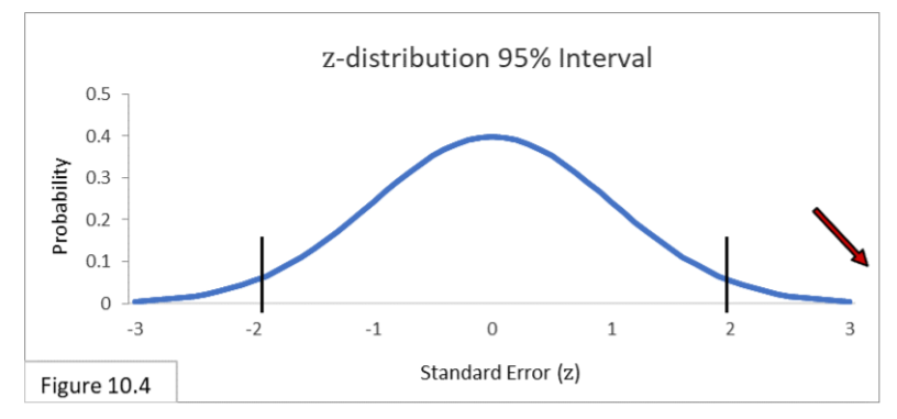
(It’s off the chart shown here, but the z-distribution itself actually goes from negative infinity to positive infinity.) With sample sizes of 1000, the difference of .08 between .52 and .44 is statistically significant, and we do reject the Null Hypothesis that Flowing Wells and Artesian Wells have equal population binomial proportions. While the .08 difference was not statistically significant in March with sample sizes of 100, it is statistically significant in May with sample sizes of 1000. The additional statistical power due to the larger sample size does that. And while it is always possible that a Type I Error has occurred whenever we reject a Null Hypothesis, our experience over the last few months convinces us that this month’s difference is most likely real. It is unclear, however, whether 52% and 44% are different enough to have serious political implications. Perhaps we need to ask some political scientists whether they think these statistically significant survey results have any practical significance.
Next: The Rest of the (Frequentist) Iceberg
References
J.E. Kotteman. Statistical Analysis Illustrated – Foundations . Published via Copyleft. You are free to copy and distribute the content of this article.