Posterior Probability & the Posterior Distribution

Probability > Posterior Probability & the Posterior Distribution

What is Posterior Probability?
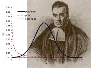
posterior probability
Posterior probabilities are used in Bayesian hypothesis testing. Image: Los Alamos National Lab.


Posterior probability is the conditional probability an event will happen after all evidence or background information has been taken into account. To put that another way: if we know the conditional and unconditional probabilities of one event in advance, we can calculate the conditional probabilities for a second event.

Posterior and prior probability are related in the following way:

Posterior probability = prior probability + new evidence 

  • Prior probability is an estimate of the likelihood that something will happen, before any new evidence has been included.
  • Posterior probability adds a layer to prior probability by factoring in new evidence (called “likelihood”) and adjusting your prior belief accordingly – it’s effectively like taking another look with fresh eyes.

To demonstrate how posterior probability works, imagine you are attempting to find out what proportion of college students finish their degree within six years. Historical records inform your prior probability at 60%. After surveying more recent graduates however, the figure may be closer to 50% – representing an adjustment via posterior probability.

Calculating Posterior Probability

Posterior probability is calculated by updating the prior probability with Bayes’ rule.

Bayes Theorem examples
The formal definition of Bayes’ Rule.

  The formula can be broken down into parts:

  • P(A|B) = posterior probability of event A.
  • P(B|A) = likelihood of event B, given that A has already happened.
  • P(A) = prior probability of event A.
  • P(B) = prior probability of event B.

For example, let’s say you wanted to find a patient’s probability of having fatty liver disease, given that they are obese. “Being obese” is the test (in the sense of a litmus test) for fatty liver disease. We know some facts about the following events:

  • Event A is the event “Patient has fatty liver disease.” Past data tells you that 10% of patients have fatty liver disease. P(A) = 0.10.
  • Event B is the test that “Patient is obese.” Five percent of the clinic’s patients are obese. P(B) = 0.05.
  • You also know that among those patients diagnosed with fatty liver disease, 7% are obese. This is B|A (B given A): the probability a patient is obese, given that they have liver disease, is 7%.

Plugging these into the Bayes’ theorem formula:

P(A|B) = (0.07 * 0.1)/0.05 = 0.14

If the patient is obese, their probability of having fatty liver disease is 0.14 (14%). This is a significant increase from the 10% suggested by past data.

Origin of the Terms

Understanding the terms posterior and prior depends on being familiar with Latin philosophical terminology – specifically, a priori. This phrase describes an intuitive knowledge that comes from understanding how principles work, rather than simply relying on observation of their results. The words posterior and prior come from the Latin posterior (“later”) and prior (“earlier”). The definition of “a priori” is similar, also stems from Latin. However, it means “from something that came before”.

Merriam Webster defines a priori as:

“…relating to what can be known through an understanding of how certain things work [i.e., a hypothesis] rather than by observation.”

By comparison, its opposite “a posteriori” emphasizes what can be determined through direct experience or observation alone.

What is a Posterior Distribution?

Bayesian Analysis is an important tool for quantifying uncertainty, and the posterior distribution lies at its heart. Given prior information combined with data from observations or experiments, the posterior summarizes all you know after factoring in that new evidence. It provides estimates of parameters like intervals or points as well as predictions about future data outcomes through probabilistic evaluations to help inform decisions under uncertain conditions.

The posterior distribution is a way to summarize what we know about uncertain quantities in Bayesian statistics. It is a combination of the prior distribution and the likelihood function, which tells you what information is contained in your observed data (the “new evidence”).

Thus, the posterior probability distribution is a compromise between the prior distribution and likelihood function. In other words, the posterior distribution summarizes what you know after the data has been observed, where the summary of the evidence from the new observations is the likelihood function.

Posterior Distribution = Prior Distribution + Likelihood Function (“new evidence”)

We can rewrite Bayes’ rule to express it in terms of probability distributions [1]: bayes theorem in terms of probability distributions Where

  • f(θ|data) = posterior distribution for parameter θ,
  • f(data|θ) = sampling density for the data. This is proportional to the likelihood function and differs only by a constant which would make it a “proper” density function,
  • (θ) = prior distribution for the parameter,
  • f(data) = the data’s marginal probability — the probability of observing the data regardless of the parameter’s value.

Posterior distributions are integral to Bayesian analysis. They are, in many ways, the goal of the analysis and can give you:

Prior vs. Posterior probability

Posterior probability is closely related to prior probability, which is the probability an event will happen before you taken any new evidence into account. You can think of posterior probability as an adjustment on prior probability:

Posterior probability = prior probability + new evidence (called ‘likelihood’)

For example, historical data suggests that around 60% of students who start college will graduate within 6 years. This is the prior probability. However, you think that figure is much lower, so you set out to collect new data. The evidence you collect suggests that the true figure is closer to 50%; This is the posterior probability.

Thus, posterior probability distributions better reflect the true probability than the prior probability because it incorporates more information.

References

[1] Basics of Bayesian Statistics


Comments? Need to post a correction? Please Contact Us.