Probability Distributions > Stable Distribution
What is a Stable Distribution?
Stable distributions are a family of probability distributions that share certain properties. They were first described by Paul Lévy in 1925 [1] and so are also sometimes called Lévy alpha-stable distributions.
A random variable is stable if you take two independent copies of a random variable, add them together, and the sum has the same distribution as the original random variable — up to the location and scale parameters. They are important because they are attractors for properly normed sums of IID random variables. This means that if you take any probability distribution sum a large number of IID random variables, the sum’s distribution will eventually converge to the attractor distribution. This important property allows us to use stable distributions to model many random phenomena such as the behavior of earthquakes or financial markets.
While Paul Lévy’s 1925 description of Stable Distributions [1] has granted them the nickname ‘Lévy distributions’, it is actually a misnomer as this simply refers to one specific member within the broader family. Nonetheless, each and every stable distribution exhibits certain shared properties that make them useful partners in probability calculations.
Most stable distributions do not have a distinct probability density function (pdf), with the exception of the Cauchy Distribution, Lévy Distribution and Normal distribution. But they do share certain properties, such as skewness and heavy tails. The pdf gives us insight into how likely certain events are to occur given certain sets of data.
The Cauchy distribution is especially interesting due to its ability to model fat-tailed phenomena such as stock market crashes and extreme weather events. The Lévy distribution is also known for its ability to model large-scale phenomena such as global sea surface temperatures or large financial transactions. Finally, the Normal distribution is probably the most well-known type of stable distribution due to its widespread use in statistical analysis and forecasting models.
Properties of Stable Distributions
The general stable distribution has four parameters [3]:
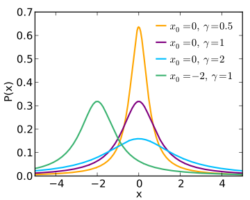
- Index of stability: (0 < α ≤ 2). This parameter determines the probability in the extreme tails (i.e., it tells you something about the behavior of the tails). A normal distribution has α = 2. Distributions below that number (i.e., with 0 < α ≤ 2) will be more heavy in the tails. The Cauchy distribution has α = 1. The stable distributions have undefined variance for α < 2, and undefined mean for α ≤ 1 [4].
- Skewness parameter (β). If β = 0, then the distribution is a symmetrical distribution. A normal distribution has β = 0.
- Scale parameter (γ). A measure of dispersion. For the normal distribution, γ = half of the population variance. For other symmetric distributions in the family, one suggestion is to exclude the top and bottom 28% of observations; By excluding the heavy tails, we can get a better estimate of γ [5].
- Location parameter: δ. This parameter equals the median. When α > 1, it also equals the mean. For a normal distribution, the sample mean can be used as an estimate for δ. For other distributions, it may be necessary to discard extreme values in order to get a good estimate for δ. Depending on how heavy the tails are, you may need to exclude the first and last quartiles — only using the central half of observations.
- One of the most important mathematical characteristics of stable distributions is that they retain the same α and β under convolution of random variables (a term which describes what happens when two functions f and g are combined to form a third function).
Alpha Stable Distribution
The alpha stable distribution is a versatile family of distributions that can be specified by four parameters, α, β, γ, and δ. These control the characterisitic exponent which determines how long the tails are; skewness to decide if its right or left skewed; scale parameter for variance similar in normal distribtion; and location shift for mean, respectively. It’s all packaged up nicely into one powerful formula with (α, β, γ, δ). An interesting way to think about it – when expressed as standard stable random variable, any other values than these will conform to this same equation through scaling/shifting combinations.
Advantages and Disadvantages for Practical Use
Stable distributions play an important role in probability calculations because they can help us understand the underlying phenomenon behind various events or outcomes. For example, if we know the pdfs associated with each type of stable distribution, then we can better predict how likely certain outcomes are given different sets of data – something that would otherwise be impossible for randomly behaving data sets without this knowledge. Furthermore, understanding how these pdfs interact with one another can help us make more accurate predictions about future events or outcomes based on past data sets. This could be invaluable information for businesses looking to plan ahead for future scenarios or investors trying to make sound financial decisions based on past trends.
Another very useful property of stable distributions is that they are scalable (up to a certain factor) — a small part of the distribution looks just like the whole.
A major drawback to the use of stable distributions is that any moment greater than α isn’t defined. That means in general, any theory based on variance (the second moment) isn’t useful. However, it’s sometimes possible to modify the distributions (for example, truncate the tails). This does require you to have a good grasp of the particular distribution you’re dealing with as well as the discipline from which your data was drawn in the first place. For example, Paul & Baschnagel [6] describe how a Lévy distribution can be used to model a human heart beat if the tails are truncated — but you would only know to truncate the tails if you were aware that deviations in heartbeats can’t be arbitrarily large.
References
- Paul Lévy(1925). Calul des probabilities.
- Image: Skbkekas | Wikimedia Commons. CC 3.0.
- Ole E. Barndorff-Nielsen, Thomas Mikosch,
- UC Davis. Lecture 12. [PPT]
- Fama, E.F. and Roll, R. (1968). Some Properties of Symmetric Stable Distributions.
- Jörg Baschnagel. Stochastic Processes: From Physics to Finance.