Inverse Distribution Function / Point Function / Quantile Function

Types of Function > Inverse Distribution Function / Point Function / Quantile Function

Contents:

1. Inverse Distribution Function Definition
   • Relationship Between CDF and Inverse Probability Function
2. Point Function
3. Percent Point Function
4. Quantile Function

Inverse Distribution Function

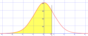
The inverse distribution function (IDF) for continuous variables F_x^-1(α) is the inverse of the cumulative distribution function (CDF). In other words, it’s simply the distribution function F_x(x) inverted. The CDF shows the probability a random variable X is found at a value equal to or less than a certain x. Intuitively, it’s how much area is under the curve at a certain point. The inversion of the CDF, the IDF, gives a value for x such that: F_X(x) = Pr(X ≤ x) = s, Where s is where random draws would fall s * 100 percent of the time [1]. The process sounds simple—invert the CDF— but many distributions don’t actually have simple inversions. The exponential distribution is one exception where the inverse is defined as:
Good approximations are available for common functions like the normal and gamma distributions.

Relationship Between CDF and Inverse Probability Function

The quantile function and the cumulative distribution function (CDF) are two different ways of describing a probability distribution:

• The quantile function takes a probability as input and give us a value for the distribution. For example, p = 0.5 would give us the median.
• The CDF takes a distribution value as input and gives us the probability of obtaining a value less than or equal to that input. For instance, a value of 0.5 would give us the probability of obtaining a value less than or equal to 0.5.

The CDF gives you probabilities of a random variable X being less than or equal to some value x. The z-table is a basic example of how this works: a score found on the table shows the probability of a random variable falling to the left of the score (the “x”):

The inverse of the CDF (i.e. the Inverse Function) tells you what value x (in this example, the z-score) would make F(x)— the normal distribution in this case— return a particular probability p. In notation, that’s: F^-1(p) = x. To sum that all up:

• CDF = what area/probability corresponds to a known z-score?
• Inverse Function = what z-score corresponds to a known area/probability?

I used the normal distribution as an example as that’s the distribution most people seem to be familiar with. However, the concept can be applied to most distributions.

Point Function

A point function is a way to define variable quantities that depend only on position for their values (for example, x, y, z). A point function can be scalar or vector.

Scalar and Vector Point Function Example

A scalar point function is defined by a set of real-valued points P(x, y, z) in a scalar field; if each point has a unique scalar, then the function is a scalar point function (sometimes called scalar function of position).

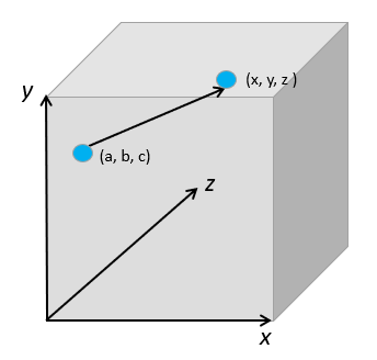
As an example, the distance of the set of all points (x, y, z) from fixed point (a, b, c) can be represented by the following scalar point function: f(p) = {(x – a)² + (y – b)² + (z – c)²}^½ Real-world scalar point functions can be used to represent a variety of physical systems, including (Taneja, 2010):

• The distribution of atmospheric pressure in space,
• Temperature distribution in a medium, or
• Density of a body.

A scalar point function is independent of the coordinate system: it only depends on the position of the point. For example, the temperature in a medium doesn’t depend on the choice of axes. If, on the other hand, each point has a corresponding vector, then the function is called a vector point function [2]. Examples of systems that can be represented by vector point functions (also called vector functions of position) include instantaneous velocity of a moving fluid, gravitational force, or electrical intensity [3]. If the direction of the axes is changed, the components will change, but the magnitude and direction will stay the same. For example, the velocity of a point in a moving fluid will be the same even if the axes are rotated [4].

Percent Point Function

The term “Percent Point Function” is usually used to denote a specific inverse function. For example,  the chi-squared distribution percent point function is used with significance level α to reject the null hypothesis. Percent point functions exist for a wide range of distributions including the gamma distribution, Weibull distribution, triangular distribution, and many more.

Quantile Function

The quantile function is equivalent to the Inverse Distribution Function or Percent Point Function. Quantile functions calculate the quantile based on a specified distribution and probability. The word quantile comes from the word quantity. It refers to dividing a probability distribution into areas of equal probability. The quantile function is equivalent to the Inverse Distribution Function or Percent Point Function. Quantile functions calculate the quantile based on a specified distribution and probability.

Before the advent of the computer, extensive tables of quantile functions were in common use. Although some of these tables can still be found in libraries, modern computing has rendered them obsolete. Nowadays, you’ll mostly come across quantile functions in software, such in SAS, where the Quantile Function returns the quantile of a distribution for a specified left probability (i.e, a CDF) [1]. Thus, you can think of a quantile function as a mathematical procedure that returns a quantile of a probability distribution, given a certain probability. For example, For example, if the probability is 0.5, then the quantile function will return the distribution’s median.

Formal definition of quantiles

Although quantiles are not always unique, it is convenient in a mathematical sense to define a function that gives us a quantile for each probability. If F is a distribution function — a function that takes a real number x as input and returns the probability that a random variable X will be less than or equal to x –, then the corresponding quantile function G will be:

G(q) = inf{ x ∈ ℝ : F(x) ≥ q },

where

• 0 < q < 1,
• inf = infimum of a set. It is the smallest element of the set — in this case, the set of all real numbers x such that F(x) ≥ q.

If the q^th quantile is unique, then it is G(q). If the q^th quantile is not unique, then G(q) is the smallest q^th quantile. The empirical quantile function is the quantile function of the empirical distribution function F_n [5]

where i — the index of the order statistic greater than or equal to p — is chosen such that

• (i – 1)/n < p ≤ i/n
• X_n(1), …, X_n(n) are the order statistics of the sample (X_n(1) ≤ … ≤ X_n(n))
• X_n(1), …, X_n(n) is a permutation (i.e., a rearrangement) of the sample X₁, …, X_{n .}

References

1. Greiner, D. et. al (2014). Advances in Evolutionary and Deterministic Methods for Design, Optimization and Control in Engineering and Sciences. Springer.
2. Kumar, V. & Jaskaran, D. (2009). Engineering Mathematics – II. Technical Publications.
3. Taneja, H. (2010). Advanced Engineering Mathematics. I.K. International Publishing House Pvt. Limited.
4. Urwin, K. (2014). Advanced Calculus and Vector Field Theory. Elsevier Science.
5. Bartlett, P. Theoretical Statistics. Lecture 20.