Contents:
What is the empirical rule (68 95 99.7 rule)?
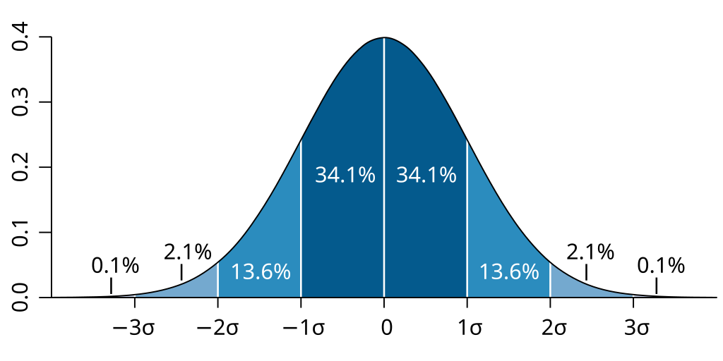
When using a normal distribution, the empirical rule, also called the 68 95 99.7 rule, the standard deviation rule, or three-sigma , tells us that:
- About 68% of values fall within one standard deviation of the mean.
- About 95% of the values fall within two standard deviations from the mean.
- Almost all of the values—about 99.7%—fall within three standard deviations from the mean.
These facts are the 68 95 99.7 rule. It is sometimes called the Empirical Rule because the rule originally came from observations (empirical means “based on observation”).
The Normal/Gaussian distribution is the most common type of data distribution. All of the measurements are computed as distances from the mean and are reported in standard deviations. The Gaussian curve is a symmetric distribution, so the middle 68.2% can be divided in two. Zero to 1 standard deviations from the mean has 34.1% of the data. The opposite side is the same (0 to -1 standard deviations). Together, this area adds up to about 68% of the data.
Thanks to the empirical rule, if you know two statistics — the mean and standard deviation — you can calculate a wide range of probabilities and percentages for various outcomes in many different types of data. The empirical rule also allows us to assess the “normality” of data. If a significant number of data points lie beyond the three standard deviation boundaries, it indicates that the distribution might not be normal and might be skewed or fit a different probability distribution.
When to use the Rule
The empirical rule is a rule of thumb that allows us to predict probabilities of large amount of data with some degree of accuracy. It helps us to estimate the percentage of data that falls within specific ranges around the mean and can help us spot outliers (unusually high or low data points). The rule can also be used to create other statistics such as:
- Confidence intervals, which indicate likely ranges containing the true value of a population parameter.
- Statistical power, defined as the probability of rejecting a false null hypothesis.
Although the empirical rule is a helpful tool for understanding how data is distributed, it is a rule of thumb and isn’t always suitable for all data. Many factors can influence how data is distributed and much of it will be beyond the empirical rule’s scope.
The empirical rule can be applied to any symmetric, unimodal distribution. The Normal distribution is the most common type of probability distribution used in elementary statistics; Many naturally occurring phenomena, such as height, weight, and IQ scores, are normally distributed.
In practice, most data sets are not normal. However, the rule can still be a useful approximation for any data set that is normal, approximately normal, bell-shaped, or unimodal (single peaked) and symmetric.
If you have data that can’t be analyzed with the empirical rule, use Chebyshev’s theorem instead. The theorem states:
For a population or sample, the proportion of observations is no less than (1 – (1 / k2 ))
While Chebyshev’s theorem allows you to calculate proportions or percentages for any distribution, it isn’t as accurate as the empirical rule for unimodal and symmetric data. Therefore, you should use the empirical rule whenever possible.
Advantages and disadvantages
The empirical rule’s advantages include:
- Simple to use.
- Applicable to a wide range of data.
- Gives us a useful tool for making predictions about where the bulk of data lies — this is especially helpful with very large populations that are challenging to analyze.
Disadvantages include:
- The rule is only an approximation and can be inaccurate.
- Exceptions can be hard to spot unless you know for certain your data fits a unimodal and symmetric distribution.
- It can be misleading if data is not normal — which can lead to overestimates or underestimates.
Empirical rule examples
Example question 1: The mean weight of new born babies at a certain general hospital is 70 lbs. with a standard deviation of 2.5 lbs. Assuming a normal distribution, answer the following questions:
- What weight is 1 standard deviation above the mean? The question tells us that the standard deviation is equal to 2.5 lbs. and the mean weight is 2.5 lbs., so a dog one standard deviation above the mean would weigh 70 lbs + 2.5 lbs = 72.5 lbs.
- What weight range covers the middle 68% of babies? The 68 95 99.7 rule states that 68% of the weights should be within one standard deviation on either side of the mean. We calculated one standard deviation above the mean in question 1: 72.5 lbs.; to find 1 standard deviation below, subtract 2.5 lbs. from the mean: 70 lbs – 2.5 lbs = 67.5 lbs. Therefore, 68% of dogs weigh between 67.5 and 72.5 lbs.
Example 2: The mean lifespan of a domestic rabbit is 10 years, with a standard deviation of 1.5 years. Apply the empirical rule to find out the lifespan of 99.7% of rabbits. Assume the data is normally distributed.
Solution: The empirical rule tells us that 99.7% of values fall within three standard deviations from the mean. We need to add and subtract three standard deviations from the mean to get the range:
- Multiply the standard deviation by 3: 1.5 + 3 = 4.5.
- Add three standard deviations to the mean: µ + 3σ = 10 + 4.5 = 14.5.
- Subtract three standard deviations from the mean: µ – 3σ = 10 – 4.5 = 5.5.
- (µ ± 3σ): 5.4 to 14.5 years
Example question 3: The weights of stray dogs at a particular pound average 70 lbs with a standard deviation of 2.5 lbs. Assuming the weights follow a Gaussian distribution:
- What weight is 2 standard deviations below the mean?
- What weight is 1 standard deviation above the mean?
- The middle 68% of dogs weigh how much?
Solutions:
- 2 standard deviations is 2 * 2.5 (5 lbs). So if a dog is 2 standard deviations below the mean they weigh 70 lbs – 5 lbs = 65 lbs.
- 1 standard deviation is 2.5 lbs, so a dog 1 standard deviation above the mean would weigh 70 lbs + 2.5 lbs = 72.5 lbs.
- The 68 95 99.7 Rule tells us that 68% of the weights should be within 1 standard deviation either side of the mean. 1 standard deviation above (given in the answer to question 2) is 72.5 lbs; 1 standard deviation below is 70 lbs – 2.5 lbs is 67.5 lbs. Therefore, 68% of dogs weigh between 67.5 and 72.5 lbs.
Real life examples using the empirical rule
The normal distribution exists in theory — and it’s the most popular distribution used for teaching statistics — but it’s not commonly found in real life [2]. Real life examples include:
- The length of the human pregnancy from conception to birth is normally distributed with a mean of 266 days and a standard deviation of 16 days [3].
- SAT scores — like most exam scores — are normally distributed, but the distribution can vary slightly from year to year. This means that you can use the empirical rule, but only as a rough approximation.
- The length of pickled gherkins: the lengths of any vegetable are often approximately normal. This may seem like trivial information, but this type of information is very important to food manufacturers, who need to know how much space x amount of gherkins will probably take up in x jars. This ensures that the company will have enough jars of hand to pickle an incoming batch of gherkins.
History of the 68 95 99.7 Rule
he 68 95 99.7 rule was first coined by Abraham de Moivre in 1733, 75 years before the normal distribution model was published. De Moivre worked in the developing field of probability. Perhaps his biggest contribution to statistics was the 1756 edition of The Doctrine of Chances, containing his work on the approximation to the binomial distribution by the normal distribution in the case of a large number of trials.
De Moivre discovered the 68 95 99.7 rule with an experiment. You can do your own experiment by flipping 100 fair coins. Note:
- How many heads you would expect to see; these are “successes” in this binomial experiment.
- The standard deviation.
- The upper and lower limits for the number of heads you would get 68% of the time, 95% of the time and 99.7% of the time
Empirical Rule & The Area Under the Curve
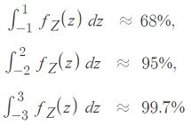
The 68-95-99.7 rule tells us the area under the curve for a normal distribution. In other words, it’s telling us values of the integral:
![]()
Where fZ(z) is the normal distribution’s pdf![]()
The integral can be evaluated for standard deviations to derive the empirical rule:
The exponential function e-z2/2 doesn’t have a simple antiderivative, so the integral has to be calculated with numerical integration. For example, as a Taylor series or with Riemann sums (Simpson’s rule is one of the better variants).
Taylor Series Steps
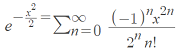
One way to define the exponential function e(x) is as a Taylor series for x = 0:
![]()
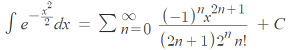
Using a little algebra, we can extend the definition to e-x2/2:
- Integrating:


- For the standard normal distribution cdf Φ, we want Φ(0) = ½:
 for x ≈ 0.
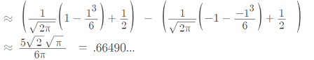
At 68%, the approximation for the empirical rule comes fairly close:
Beyond the 68 95 and 99.7 rule
Even though the empirical rule is also called the 68 95 99 rule, it isn’t limited to those percentages. You can also use it to make prediction about data’s symmetry and how the data is centered on the mean.
For example, let’s say you’re analyzing data from a package delivery service, and you know that standard delivery times average 5 days with a standard deviation of 1 day. The 68 95 99 rule tells us that 95% of delivery times will fall within the range of ±2 standard deviations, which is 5±2 = 3 to 7 days. This leaves 5% outside of this range. In other words, 5% of packages will arrive either earlier than 3 days or later than 7 days. The distribution is symmetrical, so we can extrapolate that to say that 2.5% of packages will arrive earlier than 3 days and 2.5% will arrive later than 7 days.
Using the empirical rule, we can calculate the probability of a delivery taking between 3 and 5 days — helpful if you’re planning on a gift arriving on time! As 5 is the mean, we know that 50% of packages will arrive before 5 days is up. And we also calculated that 2.5% of packages arrive before 3 days. So the probability of a package delivery taking between 3 and 5 days is 50% – 2.5% = 47.5%.
Alternatively, z-scores can be used to calculate probabilities and percentiles for data that conforms to a normal distribution.
Empirical Research Definition
The word “empirical” means based on observation or experience rather than theory. While the empirical rule is a practical “rule of thumb”, empirical research is where you conduct “hands on” experimentation. In other words, you get your results from actual experience rather than from a theory or belief.
This type of research has four major characteristics:
- A research question is posed.
- The target behavior, population, or phenomena is defined.
- The process is described in detail so that the research can be verified and duplicated. For example, a researcher might include information about any use of instruments and control groups.
Calculus forms a foundation for many quantitative research methods and is an integral part of professional empirical research.
Examples of Empirical Research:
- Pavlov’s Dog Experiments: Pavlov, most famous for his “Salivating Dogs,” actually won more acclaim for his empirical research involving the digestive system. Until Pavlov’s experiments, little was known about the digestive system. His carefully carried out and documented experiments on dogs resulted in him receiving the Nobel prize in physiology of Medicine in 1904.
- Discovery of the DNA Double Helix: Watson and Crick discovered the double helix in 19531. Until their discovery, nothing was known about the structure of the smallest unit of genetic information known at the time–the gene. After many failed model-building attempts, they finally built a model that matched the known information about the gene’s structure. The actual proof of Watson and Crick’s work came much later when laboratory experiments by several researchers (including Arthur Kornberg, Matthew Meselson, Franklin Stahl and others) confirmed their findings.
The Empirical Research Cycle
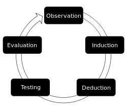
This representation of DeGroot’s empirical cycle starts with observation. We notice something, and have a question about that “something” or want to change it. That leads to induction —forming a hypothesis statement. Next is deduction, where testable consequences of the hypothesis are formulated. The actual empirical (experimental) portion of the cycle comes next, followed by evaluation of the experimental results, which leads to more questions and the beginning of the cycle.
Writing the Empirical Research paper
The IMRaD Format
Many papers (usually scientific ones) that feature empirical research have a layout called “IMRaD,” which stands for:
- Introduction: background information such as similar studies, reasons for conducting the research and any additional information necessary to understand the paper’s contents.
- Methods: details about how the experiment was conducted.
- Results: presents the results along with any statistics or analysis performed on the results.
- and
- Discussion: discusses the implications of the results.
This is the same as the APA format’ the American Psychological Association uses IMRaD headings (see the Purdue OWL website for more information on formatting in APA style).
Papers that are written for empirical research should also (no brainer here) have a title. They should also have an abstract after the title, which is a summary of the paper’s contents.
Empirical Rule & Research: References
- M. W. Toews, CC BY 2.5, via Wikimedia Commons
- UF Biostatistics. The “Normal” Shape.
- Colorado State. Applications of the Normal Distribution Solutions.
- TesseundDaan|Wikimedia. CC BY 2.5.,