Hypothesis Testing > Bartlett’s Test Contents:
What is Bartlett’s test for homogeneity of variances?
Bartlett’s test of homogeneity of variances tests the equality of variances among different samples. It checks whether the assumption of equal variances is true before certain statistical tests, such as the One-Way ANOVA, are performed.
This test is typically used when data is believed to come from a normal distribution. For non-normal distributions, Levene’s test is a more appropriate alternative. In practical terms, Bartlett’s test of homogeneity of variances can determine if any treatment variances are significantly different. A similar test, Bonferroni’s method, determines if there is any difference in means. A similar test, called Levene’s test, is a better choice for non normal distributions.
- The null hypothesis for the test is that the variances are equal for all samples. In statistics terms, that’s: H0: σ12 = σ22 = … = σk2.
- The alternate hypothesis (the one you’re testing), is that the variances are not equal for one pair or more: H0: σ12 ≠ σ22 ≠… ≠ σk2.
The test statistic is rather ugly: 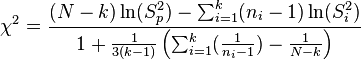
That’s why you’ll most likely want to use software for the test.
- In R, the format is [1]
- bartlett.test(x, …)
- ## Default S3 method: bartlett.test(x, g, …)
- ## S3 method for class ‘formula’ bartlett.test(formula, data, subset, na.action, …)
- Excel doesn’t have a built in function, but you can download this Bartlett’s test worksheet and fill in the blanks (Worksheet downloaded from John McDonald at The University of Delaware).
- In STATA, Bartlett’s is added onto ANOVA. The basic syntax of the command is oneway dv iv where iv is a categorical variable. For more on running the test in STATA, see this Notre Dame article.
If you really want to run Bartlett’s test by hand, follow these steps [2].
Bartlett’s Test for Equality of Variances by Hand
- The null hypothesis for the test states that the variances are equal for all samples, which in statistical notation is expressed as: H0: σ12 = σ22 = … = σk2.
- The alternate hypothesis (the one being tested) is that the variances are not equal for at least one pair: H0: σ12 ≠ σ22 ≠ … ≠ σk2.
- Calculate summary statistics (mean, variance, log of the variance, for your data.
- Calculate the pooled variance.
- Find the pooled log variances.
- Calculate q, the Bartlett statistic.
- Calculate “c”, the correction factor.
- Calculate the test statistic using the formula 2.3206(q/c)
- Find the critical chi square value. You can use a critical chi square table to do this.
- If the Bartlett test statistic from Step 6 is is greater than the critical value from Step 7, there is a significant difference in the variances.
Example: Run Barlett’s Test for Equality of Variances for the following data:
| Sample | Data Points |
|---|---|
| Sample 1 | 150, 160, 130, 170 |
| Sample 2 | 110, 130, 180, 160 |
| Sample 3 | 150, 130, 120, 160 |
| Sample 4 | 140, 170, 100, 120 |
| Sample 5 | 150, 140, 170, 190 |
Step 1: Calculate summary statistics (mean, variance, log of the variance, for your data.
Sample 1: 150, 160, 130, 170
- Mean: (150 + 160 + 130 + 170) / 4 = 152.5
- Variance: [(150 – 152.5)^2 + (160 – 152.5)^2 + (130 – 152.5)^2 + (170 – 152.5)^2] / 4 = 218.75
- Log Variance: [(log(150) – log(152.5))^2 + (log(160) – log(152.5))^2 + (log(130) – log(152.5))^2 + (log(170) – log(152.5))^2] / 4 = 0.01
Sample 2: 110, 130, 180, 160
- Mean: (110 + 130 + 180 + 160) / 4 = 145.0
- Variance: [(110 – 145)^2 + (130 – 145)^2 + (180 – 145)^2 + (160 – 145)^2] / 4 = 562.5
- Log Variance: [(log(110) – log(145))^2 + (log(130) – log(145))^2 + (log(180) – log(145))^2 + (log(160) – log(145))^2] / 4 = 0.03
Sample 3: 150, 130, 120, 160
- Mean: (150 + 130 + 120 + 160) / 4 = 140.0
- Variance: [(150 – 140)^2 + (130 – 140)^2 + (120 – 140)^2 + (160 – 140)^2] / 4 = 250.0
- Log Variance: [(log(150) – log(140))^2 + (log(130) – log(140))^2 + (log(120) – log(140))^2 + (log(160) – log(140))^2] / 4 = 0.01
Sample 4: 140, 170, 100, 120
- Mean: (140 + 170 + 100 + 120) / 4 = 132.5
- Variance: [(140 – 132.5)^2 + (170 – 132.5)^2 + (100 – 132.5)^2 + (120 – 132.5)^2] / 4 = 562.5
- Log Variance: [(log(140) – log(132.5))^2 + (log(170) – log(132.5))^2 + (log(100) – log(132.5))^2 + (log(120) – log(132.5))^2] / 4 = 0.03
Sample 5: 150, 140, 170, 190
- Mean: (150 + 140 + 170 + 190) / 4 = 162.5
- Variance: [(150 – 162.5)^2 + (140 – 162.5)^2 + (170 – 162.5)^2 + (190 – 162.5)^2] / 4 = 318.75
- Log Variance: [(log(150) – log(162.5))^2 + (log(140) – log(162.5))^2 + (log(170) – log(162.5))^2 + (log(190) – log(162.5))^2] / 4 = 0.01
Step 2: Calculate the pooled variance. The formula is:
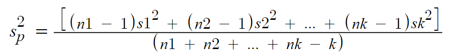
-
Calculate sample variances: (We’ve already calculated these in the previous response)
- Sample 1: 218.75
- Sample 2: 562.5
- Sample 3: 250
- Sample 4: 562.5
- Sample 5: 318.75
-
Calculate sample sizes:
- n1 = n2 = n3 = n4 = n5 = 4
-
Plug values into the pooled variance formula:
- [(4-1)*218.75 + (4-1)*562.5 + (4-1)*250 + (4-1)*562.5 + (4-1)*318.75] / (4 + 4 + 4 + 4 + 4 – 5)
- = (3*218.75 + 3*562.5 + 3*250 + 3*562.5 + 3*318.75) / 15
- = 4537.5 / 15
- = 302.5
The pooled variance for these samples is 302.5.
Step 3: Find the pooled log variances:
1. Log-transform the data:
- Sample 1: 5.0106, 5.0814, 4.8620, 5.1416
- Sample 2: 4.7005, 4.8620, 5.1929, 5.0814
- Sample 3: 5.0106, 4.8620, 4.7958, 5.0814
- Sample 4: 4.9416, 5.1416, 4.6052, 4.7958
- Sample 5: 5.0106, 4.9416, 5.1416, 5.2522
2. Calculate sample variances of the log-transformed data:
- Sample 1: 0.0103
- Sample 3: 0.0103
- Sample 4: 0.0295
- Sample 5: 0.0103
Use the pooled variance formula to calculate pooled variance for the log transformed data:
- Pooled log variance ≈ 0.0174
Step 4: Find q, the Bartlett Statistic:
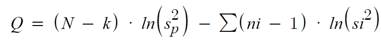
Q = (20 – 5) * ln(302.5) – 4 * (ln(218.75) + ln(562.5) + ln(250) + ln(562.5) + ln(318.75))
Q ≈ 1.8709.
Step 5: find c, the correction factor:

c ≈ 1.0333.
Step 6: Calculate the test statistic using the formula 2.3206(q/c)
2.3206(1.8709/1.0333) ≈ 4.2.
Step 7: Find the critical chi-square value:
Degrees of freedom (df):
- k = 5 (number of groups)
- df = 5 – 1 = 4
Alpha level (α):
- No level is given, so we assume α = 0.05.
Critical value:
- Using a chi-square table or software, the critical value for α = 0.05 and df = 4 is approximately 9.488.
Step 8: Compare. If the Bartlett test statistic is greater than this critical value, there is a significant difference in variances. If the statistic is less than this critical value, there is not a significance difference. For this example,
4.2 < 9.488.
Conclusion: There is not a significant difference in variances.
Bartlett’s test for Sphericity compares your correlation matrix (a matrix of Pearson correlations) to the identity matrix. In other words, it checks if there is a redundancy between variables that can be summarized with some factors.
- In IBM SPSS 22, you can find the test in the Descriptives menu: Analyse-> Dimension reduction-> Factor-> Descriptives-> KMO and Bartlett’s test of sphericity.
References
- Bartlett Test of Homogeneity of Variances. Retrieved May 18, 2023 from: https://stat.ethz.ch/R-manual/R-devel/library/stats/html/bartlett.test.html