- What is Expected Value?
- Formula
- Find an Expected Value by Hand
- Find an Expected Value in Excel
- Find an Expected Value for a Discrete Random Variable
- What is an Expected Value used for in Real Life?
- St. Petersburg Paradox
What is Expected Value?
Expected value is exactly what you might think it means intuitively: the return you can expect for some kind of action, like how many questions you might get right if you guess on a multiple choice test.
For example, if you take a 20 question multiple-choice test with A,B,C,D as the answers, and you guess all “A”, then you can expect to get 25% right (5 out of 20). The math behind this kind of expected value is:
The probability (P) of getting a question right if you guess: .25
The number of questions on the test (n)*: 20
P x n = .25 x 20 = 5
*You might see this as X instead.
This type of expected value is called an expected value for a binomial random variable. It’s a binomial experiment because there are only two possible outcomes: you get the answer right, or you get the answer wrong.
Formula
Basic Expected Value Formula
The basic expected value formula is the probability of an event multiplied by the amount of times the event happens:
(P(x) * n).
The formula changes slightly according to what kinds of events are happening. For most simple events, you’ll use either the Expected Value formula of a Binomial Random Variable or the Expected Value formula for Multiple Events.
Formula for the Expected Value of a Binomial Random Variable
The formula for the Expected Value for a binomial random variable is:
P(x) * X.
X is the number of trials and P(x) is the probability of success. For example, if you toss a coin ten times, the probability of getting a heads in each trial is 1/2 so the expected value (the number of heads you can expect to get in 10 coin tosses) is:
P(x) * X = .5 * 10 = 5
Tip: Calculate the expected value of binomial random variables (including the expected value for multiple events) using this online expected value calculator.
Expected Value for Multiple Events
Of course, calculating expected value (EV) gets more complicated in real life. For example, You buy one $10 raffle ticket for a new car valued at $15,000. Two thousand tickets are sold. What is the EV of your gain? The formula for calculating the EV where there are multiple probabilities is:
E(X) = ΣX * P(X)
Where Σ is summation notation.
The equation is basically the same, but here you are adding the sum of all the gains multiplied by their individual probabilities instead of just one probability.
Other Expected Value Formulas
The two formulas above are the two most common forms of the expected value formulas that you’ll see in AP Statistics or elementary statistics. However, in more rigorous or advanced statistics classes (like these), you might come across the expected value formulas for continuous random variables or for the expected value of an arbitrary function.
Expected Value Formula for an Arbitrary Function
Expected Value for Continuous Random Variables
The expected value of a random variable is just the mean of the random variable. You can calculate the EV of a continuous random variable using this formula:
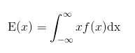
Where f(x) is the probability density function, which represents a function for the density curve.
The “∫” symbol is called an integral, and it is equivalent to finding the area under a curve.
Expected Value Formula for an Arbitrary Function
If an event is represented by a function of a random variable (g(x)) then that function is substituted into the EV for a continuous random variable formula to get:
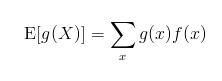
Back to Top
Calculate an Expected value in statistics by hand
This section explains how to figure out the expected value for a single item (like purchasing a single raffle ticket) and what to do if you have multiple items. If you have a discrete random variable, read Expected value for a discrete random variable.
Example question: You buy one $10 raffle ticket for a new car valued at $15,000. Two thousand tickets are sold. What is the expected value of your gain?
Step 1: Make a probability chart (see: How to construct a probability distribution). Put Gain(X) and Probability P(X) heading the rows and Win/Lose heading the columns.

Step 2: Figure out how much you could gain and lose. In our example, if we won, we’d be up $15,000 (less the $10 cost of the raffle ticket). If you lose, you’d be down $10. Fill in the data (I’m using Excel here, so the negative amounts are showing in red).

Step 3: In the bottom row, put your odds of winning or losing. Seeing as 2,000 tickets were sold, you have a 1/2000 chance of winning. And you also have a 1,999/2,000 probability chance of losing.

Step 4: Multiply the gains (X) in the top row by the Probabilities (P) in the bottom row.
$14,990 * 1/2000 = $7.495,
(-$10)*(1,999/2,000)= -$9.995
Step 5:Add the two values together:
$7.495 + -$9.995 = -$2.5.
That’s it!
Note on multiple items: for example, what if you purchase a $10 ticket, 200 tickets are sold, and as well as a car, you have runner up prizes of a CD player and luggage set?
Perform the steps exactly as above. Make a probability chart except you’ll have more items:

Then multiply/add the probabilities as in step 4: 14,990*(1/200) + 100 * (1/200) + 200 * (1/200) + -$10 * (197/200).
You’ll note now that because you have 3 prizes, you have 3 chances of winning, so your chance of losing decreases to 197/200.
Note on the formula: The actual formula for expected gain is E(X)=∑X*P(X) (this is also one of the AP Statistics formulas). What this is saying (in English) is “The expected value is the sum of all the gains multiplied by their individual probabilities.”
Like the explanation? Check out the Practically Cheating Statistics Handbook, which has hundreds more step-by-step explanations, just like this one!
Find an Expected Value in Excel
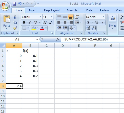
Step 1: Type your values into two columns in Excel (“x” in one column and “f(x)” in the next.
Step 2: Click an empty cell.
Step 3: Type =SUMPRODUCT(A2:A6,B2:B6) into the cell where A2:A6 is the actual location of your x variables and f(x) is the actual location of your f(x) variables.
Step 4: Press Enter.
That’s it!
Back to Top
Find an Expected Value for a Discrete Random Variable
You can think of an expected value as a mean, or average, for a probability distribution. A discrete random variable is a random variable that can only take on a certain number of values. For example, if you were rolling a die, it can only have the set of numbers {1,2,3,4,5,6}. The expected value formula for a discrete random variable is:
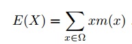
Basically, all the formula is telling you to do is find the mean by adding the probabilities. The mean and the expected value are so closely related they are basically the same thing. You’ll need to do this slightly differently depending on if you have a set of values, a set of probabilities, or a formula.
Expected Value Discrete Random Variable (given a list).
Example problem #1: The weights (X) of patients at a clinic (in pounds), are: 108, 110, 123, 134, 135, 145, 167, 187, 199. Assume one of the patients is chosen at random. What is the EV?
Step 1: Find the mean. The mean is:
108 + 110 + 123 + 134 + 135 + 145 + 167 + 187 + 199 = 145.333.
That’s it!
Expected Value Discrete Random Variable (given “X”).
Example problem #2. You toss a fair coin three times. X is the number of heads which appear. What is the EV?
Step 1: Figure out the possible values for X. For a three coin toss, you could get anywhere from 0 to 3 heads. So your values for X are 0, 1, 2 and 3.
Step 2: Figure out your probability of getting each value of X. You may need to use a sample space (The sample space for this problem is: {HHH TTT TTH THT HTT HHT HTH THH}). The probabilities are: 1/8 for 0 heads, 3/8 for 1 head, 3/8 for two heads, and 1/8 for 3 heads.
Step 3: Multiply your X values in Step 1 by the probabilities from step 2.
E(X) = 0(1/8) + 1(3/8) + 2(3/8) + 3(1/8) = 3/2.
The EV is 3/2.
Expected Value Discrete Random Variable (given a formula, f(x)).
Example problem #3. You toss a coin until a tail comes up. The probability density function is f(x) = ½x. What is the EV?
Step 1: Insert your “x” values into the first few values for the formula, one by one. For this particular formula, you’ll get:
1/20 + 1/21 + 1/22 + 1/23 + 1/24 + 1/25.
Step 2: Add up the values from Step 1:
= 1 + 1/2 + 1/4 + 1/8 + 1/16 + 1/32 = 1.96875.
Note: What you are looking for here is a number that the series converges on (i.e. a set number that the values are heading towards). In this case, the values are headed towards 2, so that is your EV.
Tip: You can only use the expected value discrete random variable formula if your function converges absolutely. In other words, the function must stop at a particular value. If it doesn’t converge, then there is no EV.
What is Expected Value in Statistics used for in Real Life?
Expected values for binomial random variables (i.e. where you have two variables) are probably the simplest type of expected values. In real life, you’re likely to encounter more complex expected values that have more than two possibilities. For example, you might buy a scratch off lottery ticket with prizes of $1000, $10 and $1. You might want to know what the payoff is going to be if you go ahead and spend $1, $5 or even $25.
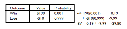
Let’s say your school is raffling off a season pass to a local theme park, and that value is $200. If the school sells one thousand $10 tickets, every person who buys the ticket will lose $9.80, expect for the person who wins the season pass. That’s a losing proposition for you (although the school will rake it in). You might want to save your money! Here’s the math behind it:
- The value of winning the season ticket is $199 (you don’t get the $10 back that you spent on the ticket.
- The odds that you win the season pass are 1 out of 1000.
- Multiply (1) by (2) to get: $199 * 0.001 = 0.199. Set this number aside for a moment.
- The odds that you lose are 999 out of 1000. In other words, your odds of ending up minus ten dollars are 999/1000. Multiplying -$10, you get -9.999.
- Adding (3) and (4) gives us the expected value: 0.199 + -9.999 = -9.80.
Here’s that scenario in a table:
St Petersburg Paradox
What is the St. Petersburg Paradox?
The St. Petersburg Paradox has been stumping mathematicians for centuries. It’s about a betting game you can always win. But despite that fact, people aren’t willing to pay much money to play it. It’s called the St. Petersburg Paradox because of where it appeared in print: in the 1738 Commentaries of the Imperial Academy of Science of Saint Petersburg.
The Paradox is this: There’s a simple betting game you can play where your winnings are always going to be bigger than the amount of money you bet. Imagine buying a scratch off lottery ticket where the expected value (i.e. the amount you can expect to win) is always higher than the amount you pay for the ticket. You could buy a ticket for $1, $10, or a million dollars. You will always come up ahead. Would you play?
Assuming the game isn’t rigged, you probably should play. But the paradox is that most people wouldn’t be willing to bet on a game like this for more than a few dollars. So, why is that? There are a couple of possible explanations:
- People aren’t rational. They aren’t willing to risk their money even for a sure bet.
- There has to be something wrong with the game’s odds. Surely the odds of winning can’t always be that good, can they?
The short answer is, people are rational (for the most part), they are willing to part with their money (for the most part). And, there is absolutely nothing wrong with the game. If you’re confused at this point — that is why it’s called a paradox.
The St. Petersburg Paradox Game.

If you figure out the expected value (the expected payoff) for this game, your potential winnings are infinite. For example, on the first flip, you have a 50% chance of winning $2. Plus you get to toss the coin again, so you also have a 25% chance of winning $4, plus a 12.5% chance of winning $8 and so on. If you bet over and over again, your expected payoff (gain) is $1 each time you play, as shown by the following table.
| P(n) | Prize | Expected payoff | |
|---|---|---|---|
| 1 | 1/2 | $2 | $1 |
| 2 | 1/4 | $4 | $1 |
| 3 | 1/8 | $8 | $1 |
| 4 | 1/16 | $16 | $1 |
| 5 | 1/32 | $32 | $1 |
| 6 | 1/64 | $64 | $1 |
| 7 | 1/128 | $128 | $1 |
| 8 | 1/256 | $256 | $1 |
| 9 | 1/512 | $512 | $1 |
| 10 | 1/1024 | $1024 | $1 |
You can’t possibly lose money. Still, despite the expected value being infinitely large, most people wouldn’t be willing to fork out more than a few bucks to play the game.
The St. Petersburg paradox has been debated by mathematicians for almost three centuries. Why won’t people risk a lot of money if the odds are certainly in their favor? As of yet, no one has found a satisfactory answer to the paradox. As Michael Clark states: “[The St. Petersburg Paradox] seems to be one of those paradoxes which we have to swallow.” A couple of solutions, which have been presented and yet have failed to offer a satisfactory answer:
- Limited utility (suggested by Jacob Bernoulli). Basically, the more we have of something, the less satisfied we are with it. You can apply this to candy; You’re likely to be satisfied with one bag, but after six or seven bags, you’re likely to not want any more. However, you can’t apply this to money. Everyone wants more money, right?
- Risk aversion. The average person might consider putting a few thousand dollars in the stock market. But they wouldn’t be willing to gamble their entire life savings. You can’t apply this rule to the St. Petersburg Paradox game because there is no risk.
Next: Powerball Expected Value
References
Clark, Michael, 2002, “The St. Petersburg Paradox”, in Paradoxes from A to Z, London: Routledge, pp. 174–177.
Papoulis, A. “Expected Value; Dispersion; Moments.” §5-4 in Probability, Random Variables, and Stochastic Processes, 2nd ed. New York: McGraw-Hill, pp. 139-152, 1984.
Related articles:
Online expected value calculator.