Probability and Statistics > Probability > Sample Space Examples
Contents:
What is a Sample Space?
The sample space of an experiment is all possible outcomes for that experiment. For example:
 |
The space for the toss of one coin: {Heads, tails.} |
 |
The space for the toss of a die: {1, 2, 3, 4, 5, 6.} |
 |
The space for choosing a card from a standard deck: {Hearts: 2, 3, 4, 5, 6, 7, 8, 9, 10, j, q, k, A. Clubs: 2, 3, 4, 5, 6, 7, 8, 9, 10, j, q, k, A. Spades: 2, 3, 4, 5, 6, 7, 8, 9, 10, j, q, k, A. Diamonds: 2, 3, 4, 5, 6, 7, 8, 9, 10, j, q, k, A.} |
 |
The sample space for the roll of TWO dice: {[1][1], [1][2], [1][3], [1][4], [1][5], [1][6], [2][1], [2][2], [2][3], [2][4],[2][5], [2][6], [3][1], [3][2], [3][3], [3][4], [3][5], [3][6], [4][1], [4][2], [4][3], [4][4], [4][5], [4][6], [5][1], [5][2], [5][3], [5][4], [5][5], [5][6], [6][1], [6][2], [6][3], [6][4], [6][5], [6][6].} |
When writing out a sample space, remember this important fact: each item in the sample space should be equally likely. In the above example, each of the 36 dice rolls is equally likely to happen. You could write the sample space another way, by just adding up the two dice. For example [1][1] = 2 and [1][2] = 3. That would give {2, 3, 4, 6, 7, 8, 9, 10, 11, 12}. But the problem is, these events aren’t equally likely. You have a 1/36 chance of rolling a 12 (6,6) and a greater chance (4/36) of rolling a seven (4,3 or 3,4 or 5,2 or 2,5).
Large Sample Spaces
The more items you throw in the mix, the more complicated it becomes. How do you make sure you don’t miss an item?
Notice how the sample space for the roll of two dice starts with the number “1” first:
[1][1], [1][2], [1][3], [1][4], [1][5], [1][6]
All of the possible combinations for the second die are listed after the number 1.
Then comes “2”:
[2][1], [2][2], [2][3], [2][4],[2][5], [2][6]
And so on. The problem is, sample spaces can get very, very large. Imagine trying to figure out the sample space for rolling six dice. There are 46656 items in the sample space! There is no fast way to make a sample space — you just have to write out all of the possibilities. However, there is a way you can figure out probabilities of choosing an item from a sample space. Rather than writing out the entire sample space, you can use the Counting Principle.
The Counting Principle
Example problem: If shoes come in 6 styles with 3 possible colors, how many varieties of shoes are there?
All you need to do is multiply: 6 • 3 = 18 possible varieties of shoes.
The Fundamental Counting Principle: If there are “a” ways for one event to happen, and “b” ways for a second event to happen, then there are “a * b” ways for both events to happen.
Examples:
- Flipping a coin and rolling a die:
There are 2 ways to flip a coin and 6 ways to roll a die, so there are 6 * 2 = 12 ways to flip a coin and roll a die. -
Drawing three cards from a standard deck without replacing the cards.
There are 52 ways to draw the first card.
There are 51 ways to draw the second card.
There are 50 ways to draw the third card.
There are 52 * 51 * 50 = 132,600 ways to draw the three cards.
You can see why you might not want to draw out the entire sample space. Can you imagine writing out all 132,600 possibilities?
The Counting Principle also works for more than two events.
-
Rolling a die four times:
There are 6 ways to roll each die.
There are 6 * 6 * 6 * 6 = 1,296 possible outcomes. - Taking a 10 question survey with 2 choices (yes or no) for each question:
There are 2 ways to answer each question.
There are 2 * 2 * 2 * 2 * 2 * 2 * 2 * 2 * 2 * 2 = 1024 ways to complete the survey.
Continuous Sample Spaces
Sample spaces introduced in early probability classes are typically discrete. That is, they are made up of a finite (fixed) amount of numbers. For example, if you roll a die, the sample space (Ω) is [1, 2, 3, 4, 5, 6]. Rolling a twenty-sided die or choosing a card from a deck all produce discrete sample spaces. A continuous sample space is based on the same principles, but it has an infinite number of items in the space. In other words, you can’t write out the space in the same way that you would write out the sample space for a die roll. With a continuous sample space, you would still be writing numbers long after the sun has imploded into a black hole.
Continuous Sample Space Example
The following image shows a continuous sample space— an area 2 units high and 2 units wide. Imagine that the space represents a game where a dart is dropped into the space and lands on a random spot. What are the odds of the dart landing on the spot pictured?
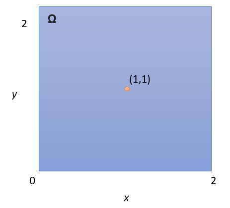
It may surprise you to learn that the odds of the ball landing on either of those two spots is zero. In fact, the odds of the dart falling in any spot at all equals zero. Let’s say the dart lands at (1, 1). It could also land a hair to the right, at (1.001, 1). Or, an even tinier fraction to the right, at (1.0000000001, 1). If you try and write down all of the possible places the dart could land, you won’t be able to, because there are an infinite number of spaces the ball could land on. If you have a problem with this logic, you aren’t alone. It’s an example of how we think the world works, and how it actually works. A famous example of how infinity messes with logic is Zeno’s paradox (also known as “&helli[;the hare can never overtake the tortoise in a race”).
A more modern approach is to use the problem in terms of limits. In simple terms, a limit is the number very close to the one you’re measuring. In the case of all these zeros (1.001, 1.0000001, 1. 00000000000001 etc.), you could say they all are very close to 1, giving you far fewer points to deal with. For the above problem, you could come up with a very reasonable probability if you could all the possible whole numbered coordinates: (0, 1), (0, 2), (0, 3) and so on.
References
Bertsekas, D. & Tsitsiklis, J. (2008). Introduction to Probability. Athena Scientific.