A pursuit curve describes a curve where one point A chases another point B. For example, a fox chasing a hen, a missile seeking a moving target, or one attack aircraft pursuing another.
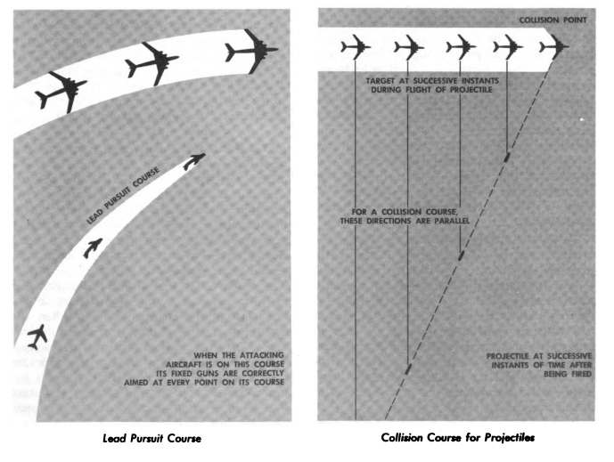
In a pure pursuit curve [2]:
- The pursuer’s velocity vector always points directly towards the pursued (i.e., point A always heads towards point B).
- Point A’s speed is proportional to point B’s speed. In other words, if point A slows down (or speeds up), then point B slows down (or speeds up).
The curve of pursuit is the curve traced by the pursuer, point A.
Pursuit Curves and Differential Equations
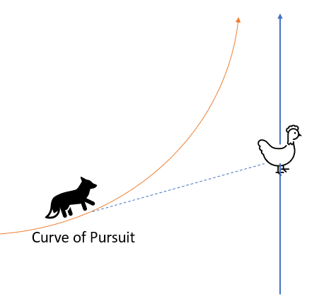
Using the analogy of a Fox (F) chasing a hen (H), and knowing that the Fox always looks at then hen (i.e., the hen is always in the tangent vector of the fox), we can describe the pursuit curve with the following equation:
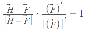
If we assume the fox has constant velocity, we can assume that

This allows us to define a system of differential equations to find a solution for the coordinates of the pursuit curve.
Difficulties with Solving the Equations
Finding solutions to pursuits can be extremely challenging. If you are able to figure out an explicit differential equation for the path of the pursuer, it will be a second order differential equation. Even relatively simple paths of pursuit can contain nodes and double points.
As an example of the difficulty in finding a solution, we can define an equation for a pursuit curve with a set of Cartesian or polar coordinates (ε, η) [3]:
f(ε, η) = 0.
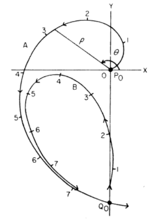
An initial point P0 is chosen as the starting point of the pursuer, and a second point Q0 designates the starting point of the pursued. This next figure shows the curve of pursuit as the parabola y2 = 4x. In this example (from the U.S. Atomic Commission [3]), both curves become asymptotesand no “capture” is achieved:
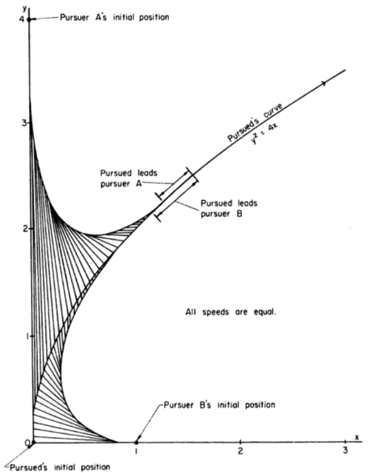
In this second example of an asymptotic path shown below, the ratio of velocities is 1. The pursuer will still never catch their prey — even if the pursuer chooses to stay in the advantageous location of where the pursued’s curve crosses the y-axis (However, if the ratio of velocities is >, the pursuer will catch their prey).
History of the Pursuit Curve
George Boole first defined the term “pursuit curve” in his 1859 work Treatise on differential equations [4]. However, he wasn’t the first to study the curves. That honor is sometimes attributed to Pierre Bouger, who formulated what is thought to be the first pursuit problem — involving a pirate ship chasing a merchant vessel — in the 1732 Memoires de l’Academie Royale des Sciences [5]. Leonardo da Vinci also studied pursuit curves, but only with regard to movement along a straight line.
References
[1] U.S. Air Force Manual, Volume 335, Issue 25. PDF.
[2] Spree. Retrieved March 3, 2022 from: http://pi.math.cornell.edu/~numb3rs/blanco/Spree.html
[3] Thayer Davis, H. U.S. Atomic Energy Commission. Introduction_to_Nonlinear_Differential Equations. PDF.
[4] Lloyd, M. (2006-07) Pursuit Curves. Retrieved March 3, 2022 from: hsu.edu/uploads/pages/2006-7afpursuit.pdf
[5] Severdia, M. (2008), Pursuit Curves. Retrieved March 3, 2022 from: https://mse.redwoods.edu/darnold/math55/DEproj/sp08/mseverdia/pursuit.pdf